Definition. Matrix size m´n, where m is the number of rows, n is the number of columns, is called a table of numbers arranged in a certain order. These numbers are called matrix elements. The location of each element is uniquely determined by the number of the row and column at the intersection of which it is located. The elements of the matrix are denoted by a ij, where i is the row number and j is the column number.
Basic operations on matrices.
A matrix can consist of either one row or one column. Generally speaking, a matrix can even consist of one element.
Definition. If the number of matrix columns is equal to the number of rows (m=n), then the matrix is called square.
Definition. If = , then the matrix is called symmetrical.
Example.- symmetric matrix
Definition. A square matrix of the form is called diagonal matrix.
Definition. A diagonal matrix with only ones on the main diagonal:
= E, called identity matrix.
Definition. A matrix that has only zero elements under its main diagonal is called upper triangular matrix. If a matrix has only zero elements above the main diagonal, then it is called lower triangular matrix.
Definition. The two matrices are called equal, if they are of the same dimension and the equality holds:
· Addition and subtraction matrices is reduced to the corresponding operations on their elements. The most important property of these operations is that they defined only for matrices of the same size. Thus, it is possible to define matrix addition and subtraction operations:
Definition. Sum (difference) matrices is a matrix whose elements are, respectively, the sum (difference) of the elements of the original matrices.
C = A + B = B + A.
· Operation multiplication (division) matrix of any size by an arbitrary number is reduced to multiplying (dividing) each element of the matrix by this number.
a (A+B) =aA ± aB
A(a±b) = aA ± bA
Example. Given matrices A = ; B = , find 2A + B.
2A = , 2A + B = .
· Definition: The work matrices is a matrix whose elements can be calculated using the following formulas:
From the above definition it is clear that the operation of matrix multiplication is defined only for matrices the number of columns of the first of which is equal to the number of rows of the second.
Example.
· Definition. Matrix B is called transposed matrix A, and the transition from A to B transposition, if the elements of each row of matrix A are written in the same order in the columns of matrix B.
A = ; B = A T = ;
in other words, = .
inverse matrix.
Definition. If there are square matrices X and A of the same order satisfying the condition:
where E is the identity matrix of the same order as the matrix A, then the matrix X is called reverse to the matrix A and is denoted by A -1.
Every square matrix with a nonzero determinant has an inverse matrix, and only one.
inverse matrix
Can be built according to the following scheme:
If , then the matrix is called non-degenerate, and otherwise – degenerate.
The inverse matrix can only be constructed for non-singular matrices.
Properties of inverse matrices.
1) (A -1) -1 = A;
2) (AB) -1 = B -1 A -1
3) (A T) -1 = (A -1) T .
Matrix rank is the highest order of the nonzero minors of this matrix.
In a matrix of order m´n, the minor of order r is called basic, if it is not equal to zero, and all minors are of order r+1 and above are equal to zero, or do not exist at all, i.e. r matches the smaller of the numbers m or n.
The columns and rows of a matrix on which the basis minor stands are also called basic.
A matrix can have several different basis minors that have the same order.
A very important property of elementary matrix transformations is that they do not change the rank of the matrix.
Definition. The matrices obtained as a result of an elementary transformation are called equivalent.
It should be noted that equal matrices and equivalent matrices are completely different concepts.
Theorem. The largest number of linearly independent columns in a matrix is equal to the number of linearly independent rows.
Because elementary transformations do not change the rank of the matrix, then the process of finding the rank of the matrix can be significantly simplified.
Example. Determine the rank of the matrix.
Note that matrix elements can be not only numbers. Let's imagine that you are describing the books that are on your bookshelf. Let your shelf be in order and all books be in strictly defined places. The table, which will contain a description of your library (by shelves and the order of books on the shelf), will also be a matrix. But such a matrix will not be numeric. Another example. Instead of numbers there are different functions, united by some dependence. The resulting table will also be called a matrix. In other words, a Matrix is any rectangular table made up of homogeneous elements. Here and further we will talk about matrices made up of numbers.
Instead of parentheses, square brackets or straight double vertical lines are used to write matrices
 |
(2.1*) |
Definition 2. If in the expression(1) m = n, then they talk about square matrix, and if , then oh rectangular.
Depending on the values of m and n, some special types of matrices are distinguished:

The most important characteristic square matrix is her determinant or determinant, which is made up of matrix elements and is denoted

Obviously, D E =1; .
Definition 3. If , then the matrix A called non-degenerate or not special.
Definition 4. If detA = 0 , then the matrix A called degenerate or special.
Definition 5. Two matrices A And B are called equal and write A = B if they have the same dimensions and their corresponding elements are equal, i.e..
For example, matrices and are equal, because they are equal in size and each element of one matrix is equal to the corresponding element of the other matrix. But the matrices cannot be called equal, although the determinants of both matrices are equal, and the sizes of the matrices are the same, but not all elements located in the same places are equal. The matrices are different because they have different sizes. The first matrix is 2x3 in size, and the second is 3x2. Although the number of elements is the same - 6 and the elements themselves are the same 1, 2, 3, 4, 5, 6, but they are in different places in each matrix. But the matrices are equal, according to Definition 5.
Definition 6. If you fix a certain number of matrix columns A and the same number of rows, then the elements at the intersection of the indicated columns and rows form a square matrix n- th order, the determinant of which called minor k – th order matrix A.
Example. Write down three second-order minors of the matrix

Matrices. Types of matrices. Operations on matrices and their properties.
Determinant of an nth order matrix. N, Z, Q, R, C,
A matrix of order m*n is a rectangular table of numbers containing m-rows and n-columns.
Matrix equality:
Two matrices are said to be equal if the number of rows and columns of one of them is equal to the number of rows and columns of the other, respectively. The elements of these matrices are equal.
Note: E-mails having the same indexes are corresponding.
Types of matrices:
Square matrix: A matrix is called square if the number of its rows is equal to the number of columns.
Rectangular: A matrix is called rectangular if the number of rows is not equal to the number of columns.
Row matrix: a matrix of order 1*n (m=1) has the form a11,a12,a13 and is called a row matrix.
Matrix column:………….
Diagonal: The diagonal of a square matrix, going from the upper left corner to the lower right corner, that is, consisting of elements a11, a22...... is called the main diagonal. (definition: a square matrix whose elements are all zero, except those located on the main diagonal, is called a diagonal matrix.
Identity: A diagonal matrix is called identity matrix if all elements are located on the main diagonal and are equal to 1.
Upper triangular: A=||aij|| is called an upper triangular matrix if aij=0. Provided i>j.
Lower triangular: aij=0. i Zero: this is a matrix whose values are equal to 0. Operations on matrices. 1.Transposition. 2.Multiplying a matrix by a number. 3. Addition of matrices. 4.Matrix multiplication. Basic properties of actions on matrices. 1.A+B=B+A (commutativity) 2.A+(B+C)=(A+B)+C (associativity) 3.a(A+B)=aA+aB (distributivity) 4.(a+b)A=aA+bA (distributive) 5.(ab)A=a(bA)=b(aA) (asoc.) 6.AB≠BA (no comm.) 7.A(BC)=(AB)C (associat.) – executed if defined. Matrix products are performed. 8.A(B+C)=AB+AC (distributive) (B+C)A=BA+CA (distributive) 9.a(AB)=(aA)B=(aB)A Determinant of a square matrix – definition and its properties. Decomposition of the determinant into rows and columns. Methods for calculating determinants. If matrix A has order m>1, then the determinant of this matrix is a number. The algebraic complement Aij of the aij element of matrix A is the minor Mij multiplied by the number THEOREM 1: The determinant of matrix A is equal to the sum of the products of all elements of an arbitrary row (column) by their algebraic complements. Basic properties of determinants. 1. The determinant of a matrix will not change when it is transposed. 2. When rearranging two rows (columns), the determinant changes sign, but its absolute value does not change. 3. The determinant of a matrix that has two identical rows (columns) is equal to 0. 4. When a row (column) of a matrix is multiplied by a number, its determinant is multiplied by this number. 5. If one of the rows (columns) of the matrix consists of 0, then the determinant of this matrix is equal to 0. 6. If all elements of the i-th row (column) of a matrix are presented as the sum of two terms, then its determinant can be represented as the sum of the determinants of two matrices. 7. The determinant will not change if the elements of one column (row) are added to the elements of another column (row), respectively, after multiplying. for the same number. 8. The sum of arbitrary elements of any column (row) of the determinant by the corresponding algebraic complement of the elements of another column (row) is equal to 0. https://pandia.ru/text/78/365/images/image004_81.gif" width="46" height="27"> Methods for calculating the determinant: 1. By definition or Theorem 1. 2. Reduction to triangular form. Definition and properties of an inverse matrix. Calculation of the inverse matrix. Matrix equations. Definition: A square matrix of order n is called the inverse of matrix A of the same order and is denoted In order for matrix A to have an inverse matrix, it is necessary and sufficient that the determinant of matrix A be different from 0. Properties of an inverse matrix: 1. Uniqueness: for a given matrix A, its inverse is unique. 2. matrix determinant 3. The operation of taking transposition and taking the inverse matrix. Matrix equations: Let A and B be two square matrices of the same order. https://pandia.ru/text/78/365/images/image008_56.gif" width="163" height="11 src="> The concept of linear dependence and independence of matrix columns. Properties of linear dependence and linear independence of a column system. Columns A1, A2...An are called linearly dependent if there is a non-trivial linear combination of them equal to the 0th column. Columns A1, A2...An are called linearly independent if there is a non-trivial linear combination of them equal to the 0th column. A linear combination is called trivial if all coefficients C(l) are equal to 0 and non-trivial otherwise. https://pandia.ru/text/78/365/images/image010_52.gif" width="88" height="24"> 2. In order for the columns to be linearly dependent, it is necessary and sufficient that some column be a linear combination of other columns. Let 1 of the columns https://pandia.ru/text/78/365/images/image014_42.gif" width="13" height="23 src=">be a linear combination of other columns. https://pandia.ru/text/78/365/images/image016_38.gif" width="79" height="24"> are linearly dependent, then all columns are linearly dependent. 4. If a system of columns is linearly independent, then any of its subsystems is also linearly independent. (Everything that is said about columns is also true for rows). Matrix minors. Basic minors. Matrix rank. Method of bordering minors for calculating the rank of a matrix. A minor of order k of a matrix A is a determinant whose elements are located at the intersection of the k-rows and k-columns of the matrix A. If all minors of the kth order of the matrix A = 0, then any minor of order k+1 is also equal to 0. Basic minor. The rank of a matrix A is the order of its basis minor. Method of bordering minors: - Select a non-zero element of matrix A (If such an element does not exist, then rank A = 0) We border the previous 1st order minor with a 2nd order minor. (If this minor is not equal to 0, then the rank is >=2) If the rank of this minor is =0, then we border the selected 1st order minor with other 2nd order minors. (If all minors of the 2nd order = 0, then the rank of the matrix = 1). Matrix rank. Methods for finding the rank of a matrix. The rank of a matrix A is the order of its basis minor. Calculation methods: 1) Method of bordering minors: - Select a non-zero element of matrix A (if there is no such element, then rank = 0) - Border the previous 1st order minor with a 2nd order minor..gif" width="40" height="22" >r+1 Mr+1=0. 2) Reducing the matrix to a stepwise form: this method is based on elementary transformations. During elementary transformations, the rank of the matrix does not change. The following transformations are called elementary transformations: Rearranging two rows (columns). Multiplying all elements of a certain column (row) by a number not =0. Adding to all elements of a certain column (row) the elements of another column (row), previously multiplied by the same number. The theorem on the basis minor. A necessary and sufficient condition for the determinant to be equal to zero. The basis minor of a matrix A is the minor of the highest kth order different from 0. The basis minor theorem: The underlying rows (columns) are linearly independent. Any row (column) of matrix A is a linear combination of the basis rows (columns). Notes: Rows and columns at the intersection of which there is a basis minor are called basis rows and columns, respectively. a11 a12… a1r a1j a21 a22….a2r a2j a31 a32….a3r a3j ar1 ar2….arr arj ak1 ak2…..akr akj Necessary and sufficient conditions for the determinant to be equal to zero: In order for a determinant of nth order to =0, it is necessary and sufficient that its rows (columns) be linearly dependent. Systems of linear equations, their classification and notation forms. Cramer's rule. Consider a system of 3 linear equations with three unknowns: https://pandia.ru/text/78/365/images/image020_29.gif" alt="l14image048" width="64" height="38 id=">!} is called the determinant of the system. Let's compose three more determinants as follows: replace sequentially 1, 2 and 3 columns in the determinant D with a column of free terms https://pandia.ru/text/78/365/images/image022_23.gif" alt="l14image052" width="93" height="22 id=">!} Proof. So, let's consider a system of 3 equations with three unknowns. Let's multiply the 1st equation of the system by the algebraic complement A11 of the element a11, the 2nd equation by A21 and the 3rd by A31: https://pandia.ru/text/78/365/images/image024_24.gif" alt="l14image056" width="247" height="31 id=">!} Let's look at each of the brackets and the right side of this equation. By the theorem on the expansion of the determinant in elements of the 1st column https://pandia.ru/text/78/365/images/image026_23.gif" alt="l14image060" width="324" height="42 id=">!} Similarly, it can be shown that and . Finally, it is easy to notice that Thus, we obtain the equality: . Hence, . The equalities and are derived similarly, from which the statement of the theorem follows. Systems of linear equations. Condition for compatibility of linear equations. Kronecker-Capelli theorem. A solution to a system of algebraic equations is such a set of n numbers C1, C2, C3......Cn, which, when substituted into the original system in place of x1, x2, x3.....xn, turns all equations of the system into identities. A system of linear algebraic equations is called consistent if it has at least one solution. A consistent system is called determinate if it has a unique solution, and indefinite if it has infinitely many solutions. Consistency conditions for systems of linear algebraic equations. a11 a12 ……a1n x1 b1 a21 a22 ……a2n x2 b2 ……………….. .. = .. am1 am2…..amn xn bn THEOREM: In order for a system of m linear equations with n unknowns to be consistent, it is necessary and sufficient that the rank of the extended matrix be equal to the rank of matrix A. Note: This theorem only provides criteria for the existence of a solution, but does not indicate a method for finding a solution. 10 question. Systems of linear equations. The basis minor method is a general method for finding all solutions to systems of linear equations. A=a21 a22…..a2n Basic minor method: Let the system be consistent and RgA=RgA’=r. Let the basis minor be written in the upper left corner of the matrix A. https://pandia.ru/text/78/365/images/image035_20.gif" width="22" height="23 src=">......gif" width="23" height="23 src= ">…...gif" width="22" height="23 src=">......gif" width="46" height="23 src=">-…..-a d2 b2-a(2r+1)x(r+1)-..-a(2n)x(n) … = ………….. Dr br-a(rr+1)x(r+1)-..-a(rn)x(n) https://pandia.ru/text/78/365/images/image050_12.gif" width="33" height="22 src="> Notes: If the rank of the main matrix and the matrix under consideration is equal to r=n, then in this case dj=bj and the system has a unique solution. Homogeneous systems of linear equations. A system of linear algebraic equations is called homogeneous if all its free terms are equal to zero. AX=0 – homogeneous system. AX =B is a heterogeneous system. Homogeneous systems are always consistent. X1 =x2 =..=xn =0 Theorem 1. Homogeneous systems have inhomogeneous solutions when the rank of the system matrix is less than the number of unknowns. Theorem 2. A homogeneous system of n-linear equations with n-unknowns has a non-zero solution when the determinant of matrix A is equal to zero. (detA=0) Properties of solutions of homogeneous systems. Any linear combination of a solution to a homogeneous system is itself a solution to this system. α1C1 +α2C2 ; α1 and α2 are some numbers. A(α1C1 +α2C2) = A(α1C1) +A(α2C2) = α1(A C1) + α2(AC2) = 0, i.e. k. (A C1) = 0; (AC2) = 0 For an inhomogeneous system this property does not hold. Fundamental system of solutions. Theorem 3. If the rank of a matrix system of an equation with n-unknowns is equal to r, then this system has n-r linearly independent solutions. Let the base minor be in the upper left corner. If r< n, то неизвестные х r+1;хr+2;..хn называются свободными переменными, а систему уравнений АХ=В запишем, как Аr Хr =Вr C1 = (C11 C21 .. Cr1 , 1,0..0) C2 = (C21 C22 .. C2r,0, 1..0)<= Линейно-независимы. …………………….. Cn-r = (Cn-r1 Cn-r2 .. Cn-rr ,0, 0..1) A system of n-r linearly independent solutions to a homogeneous system of linear equations with n-unknowns of rank r is called a fundamental system of solutions. Theorem 4. Any solution to a system of linear equations is a linear combination of a solution to the fundamental system. С = α1C1 +α2C2 +.. + αn-r Cn-r If r Question 12. General solution of a heterogeneous system. Sleep (general heterogeneous) = Coo + Sch (particular) AX=B (heterogeneous system); AX= 0 (ASoo) + ASch = ASch = B, because (ASoo) = 0 Sleep= α1C1 +α2C2 +.. + αn-r Cn-r + Sch Gauss method. This is a method of sequential elimination of unknowns (variables) - it consists in the fact that, with the help of elementary transformations, the original system of equations is reduced to an equivalent system of a stepwise form, from which all other variables are found sequentially, starting with the last variables. Let a≠0 (if this is not the case, then this can be achieved by rearranging the equations). 1) we exclude the variable x1 from the second, third...nth equation, multiplying the first equation by suitable numbers and adding the results obtained to the 2nd, 3rd...nth equation, then we get: We obtain a system equivalent to the original one. 2) exclude the variable x2 3) exclude the variable x3, etc. Continuing the process of sequentially eliminating the variables x4;x5...xr-1 we obtain for the (r-1)th step. The number zero of the last n-r in the equations means that their left side has the form: 0x1 +0x2+..+0xn If at least one of the numbers br+1, br+2... is not equal to zero, then the corresponding equality is contradictory and system (1) is not consistent. Thus, for any consistent system this br+1 ... bm is equal to zero. The last n-r equation in the system (1;r-1) are identities and can be ignored. There are two possible cases: a) the number of equations of the system (1;r-1) is equal to the number of unknowns, i.e. r=n (in this case the system has a triangular form). b)r The transition from system (1) to the equivalent system (1;r-1) is called the direct move of the Gaussian method. Finding a variable from the system (1;r-1) is the reverse of the Gaussian method. It is convenient to carry out Gaussian transformations by performing them not with equations, but with an extended matrix of their coefficients. Question 13. Similar matrices. We will consider only square matrices of order n/ A matrix A is said to be similar to matrix B (A~B) if there exists a non-singular matrix S such that A=S-1BS. Properties of similar matrices. 1) Matrix A is similar to itself. (A~A) If S=E, then EAE=E-1AE=A 2) If A~B, then B~A If A=S-1ВS => SAS-1= (SS-1)B(SS-1)=B 3) If A~B and at the same time B~C, then A~C It is given that A=S1-1BS1, and B=S2-1CS2 => A= (S1-1 S2-1) C(S2 S1) = (S2 S1)-1C(S2 S1) = S3-1CS3, where S3 = S2S1 4) The determinants of similar matrices are equal. Given that A~B, it is necessary to prove that detA=detB. A=S-1 BS, detA=det(S-1 BS)= detS-1* detB* detS = 1/detS *detB*detS (reduced) = detB. 5) The ranks of similar matrices coincide. Eigenvectors and eigenvalues of matrices. The number λ is called an eigenvalue of matrix A if there is a non-zero vector X (matrix column) such that AX = λ X, vector X is called an eigenvector of matrix A, and the set of all eigenvalues is called the spectrum of matrix A. Properties of eigenvectors. 1) When multiplying an eigenvector by a number, we obtain an eigenvector with the same eigenvalue. AX = λ X; X≠0 α X => A(α X) = α (AX) = α(λ X) = = λ (αX) 2) Eigenvectors with pairwise different eigenvalues are linearly independent λ1, λ2,.. λk. Let the system consist of 1 vector, let’s take an inductive step: С1 Х1 +С2 Х2 + .. +Сn Хn = 0 (1) – multiply by A. C1 AX1 +C2 AX2 + .. +Cn AXn = 0 С1 λ1 Х1 +С2 λ2 Х2 + .. +Сn λn Хn = 0 Multiply by λn+1 and subtract С1 Х1 +С2 Х2 + .. +Сn Хn+ Сn+1 Хn+1 = 0 С1 λ1 Х1 +С2 λ2 Х2 + .. +Сn λn Хn+ Сn+1 λn+1 Хn+1 = 0 C1 (λ1 –λn+1)X1 + C2 (λ2 –λn+1)X2 +.. + Cn (λn –λn+1)Xn + Cn+1 (λn+1 –λn+1)Xn+1 = 0 C1 (λ1 –λn+1)X1 + C2 (λ2 –λn+1)X2 +.. + Cn (λn –λn+1)Xn = 0 It is necessary that C1 = C2 =... = Cn = 0 Сn+1 Хn+1 λn+1 =0 Characteristic equation. A-λE is called the characteristic matrix for matrix A. In order for a non-zero vector X to be an eigenvector of the matrix A, corresponding to the eigenvalue λ, it is necessary that it be a solution to a homogeneous system of linear algebraic equations (A - λE)X = 0 The system has a nontrivial solution when det (A - XE) = 0 - this is the characteristic equation. Statement! The characteristic equations of such matrices coincide. det(S-1AS – λE) = det(S-1AS – λ S-1ЕS) =det(S-1 (A – λE)S) = det S-1 det(A – λE) detS= det(A – λE) Characteristic polynomial. det(A – λE) - function relative to the parameter λ det(A – λE) = (-1)n Xn +(-1)n-1(a11+a22+..+ann)λn-1+..+detA This polynomial is called the characteristic polynomial of matrix A. Consequence: 1) If the matrices are A~B, then the sum of their diagonal elements coincides. a11+a22+..+ann = в11+в22+..+вnn 2) The set of eigenvalues of similar matrices coincide. If the characteristic equations of the matrices coincide, then they are not necessarily similar. For matrix A For matrix B https://pandia.ru/text/78/365/images/image062_10.gif" width="92" height="38"> Det(Ag-λE) = (λ11 – λ)(λ22 – λ)…(λnn – λ)= 0 In order for a matrix A of order n to be diagonalizable, it is necessary that there exist linearly independent eigenvectors of the matrix A. Consequence. If all the eigenvalues of a matrix A are different, then it is diagonalizable. Algorithm for finding eigenvectors and eigenvalues. 1) compose a characteristic equation 2) find the roots of the equations 3) we compose a system of equations to determine the eigenvector. λi (A-λi E)X = 0 4) find a fundamental system of solutions x1,x2..xn-r, where r is the rank of the characteristic matrix. r =Rg(A - λi E) 5) eigenvector, eigenvalues λi are written as: X = С1 Х1 +С2 Х2 + .. +Сn-r Хn-r, where С12 +С22 +… С2n ≠0 6) check whether the matrix can be reduced to diagonal form. 7) find Ag Ag = S-1AS S= Question 15. The basis of a straight line, plane, space. https://pandia.ru/text/78/365/images/image065_9.gif" height="11">│, ││). The modulus of a vector is zero when this vector is zero (│ō│=0) 4. Orth vector. An orth of a given vector is a vector that has the same direction as the given vector and has a modulus equal to one. Equal vectors have equal vectors. 5.Angle between two vectors. This is a smaller part of the area, limited by two rays emanating from the same point and directed in the same way with the given vectors. Vector addition. Multiplying a vector by a number. 1) Addition of two vectors https://pandia.ru/text/78/365/images/image065_9.gif" height="11">+ │≤│ │+│ │ 2)Multiplying a vector by a scalar. The product of a vector and a scalar is a new vector that has: a) = product of the modulus of the vector being multiplied by the absolute value of the scalar. b) the direction is the same as the vector being multiplied if the scalar is positive, and opposite if the scalar is negative. λ а(vector)=>│ λ │= │ λ │=│ λ ││ │ Properties of linear operations on vectors. 1. The law of communicability. 2. Law of associativity. 3. Addition with zero. a(vector)+ō= a(vector) 4. Addition with the opposite. 5. (αβ) = α(β) = β(α) 6;7.The law of distributivity. Expressing a vector in terms of its modulus and orth. The maximum number of linearly independent vectors is called a basis. A basis on a line is any non-zero vector. A basis on the plane is any two non-callenary vectors. A basis in space is a system of any three non-coplanar vectors. The coefficient of expansion of a vector over a certain basis is called the components or coordinates of the vector in this basis. https://pandia.ru/text/78/365/images/image075_10.gif" height="11 src=">.gif" height="11 src="> perform the action of addition and multiplication by a scalar, then as a result any number of such actions we get: λ1 https://pandia.ru/text/78/365/images/image079_10.gif" height="11 src=">+...gif" height="11 src=">.gif" height="11 src="> are called linearly dependent if there is a nontrivial linear combination of them equal to ō. λ1 https://pandia.ru/text/78/365/images/image079_10.gif" height="11 src=">+...gif" height="11 src=">.gif" height="11 src="> are called linearly independent if there is no non-trivial linear combination of them. Properties of linearly dependent and independent vectors: 1) a system of vectors containing a zero vector is linearly dependent. λ1 https://pandia.ru/text/78/365/images/image079_10.gif" height="11 src=">+...gif" height="11 src=">.gif" height="11 src="> were linearly dependent, it is necessary that some vector be a linear combination of other vectors. 3) if some of the vectors from the system a1(vector), a2(vector)... ak(vector) are linearly dependent, then all vectors are linearly dependent. 4) if all vectors https://pandia.ru/text/78/365/images/image076_9.gif" height="11 src=">.gif" width="75" height="11"> https://pandia.ru/text/78/365/images/image082_10.gif" height="11 src=">.gif" height="11 src=">) Linear operations in coordinates. https://pandia.ru/text/78/365/images/image069_9.gif" height="12 src=">.gif" height="11 src=">.gif" height="11 src="> .gif" height="11 src=">.gif" width="65" height="13 src="> Properties of the dot product: 1. Commutativity 3. (a;b)=0, if and only if the vectors are orthoganal or some of the vectors is equal to 0. 4. Distributivity (αa+βb;c)=α(a;c)+β(b;c) 5. Expression of the scalar product of a and b in terms of their coordinates https://pandia.ru/text/78/365/images/image093_8.gif" width="40" height="11 src="> https://pandia.ru/text/78/365/images/image095_8.gif" width="254" height="13 src="> When condition () is met, h, l=1,2,3 https://pandia.ru/text/78/365/images/image098_7.gif" width="176" height="21 src="> https://pandia.ru/text/78/365/images/image065_9.gif" height="11"> and the third vector is called which satisfies the following equations: 3. – right Properties of a vector product: 4. Vector product of coordinate unit vectors Orthonormal basis. https://pandia.ru/text/78/365/images/image109_7.gif" width="41" height="11 src="> https://pandia.ru/text/78/365/images/image111_8.gif" width="41" height="11 src="> Often 3 symbols are used to denote unit vectors of an orthonormal basis https://pandia.ru/text/78/365/images/image063_10.gif" width="77" height="11 src="> https://pandia.ru/text/78/365/images/image114_5.gif" width="549" height="32 src="> If is an orthonormal basis, then https://pandia.ru/text/78/365/images/image117_5.gif" width="116" height="15">- equation of a straight line parallel to the OX axis 2) - equation of a straight line parallel to the axis of the op-amp 2. Reciprocal arrangement of 2 straight lines. Theorem 1 Let the equations of straight lines be given with respect to an affine coordinate system A) Then the necessary and sufficient condition for when they intersect has the form: B) Then the necessary and sufficient condition for the fact that the lines are parallel is the condition: B) Then a necessary and sufficient condition for the fact that the lines merge into one is the condition: 3. Distance from a point to a line. Theorem. Distance from a point to a line relative to the Cartesian coordinate system: https://pandia.ru/text/78/365/images/image127_7.gif" width="34" height="11 src="> 4. Angle between two straight lines. Perpendicularity condition. Let 2 straight lines be defined relative to the Cartesian coordinate system by general equations. https://pandia.ru/text/78/365/images/image133_4.gif" width="103" height="11 src="> If , then the lines are perpendicular. Question 24. Plane in space. Condition for vector and plane to be consistent. Distance from a point to a plane. The condition of parallelism and perpendicularity of two planes. 1. Condition for the vector and the plane to be consistent. https://pandia.ru/text/78/365/images/image138_6.gif" width="40" height="11 src="> https://pandia.ru/text/78/365/images/image140.jpg" alt="Nameless4.jpg" width="111" height="39">!} https://pandia.ru/text/78/365/images/image142_6.gif" width="86" height="11 src="> https://pandia.ru/text/78/365/images/image144_6.gif" width="148" height="11 src="> https://pandia.ru/text/78/365/images/image145.jpg" alt="Nameless5.jpg" width="88" height="57">!} https://pandia.ru/text/78/365/images/image147_6.gif" width="31" height="11 src="> https://pandia.ru/text/78/365/images/image148_4.gif" width="328" height="24 src="> 3. Angle between 2 planes. Perpendicularity condition. https://pandia.ru/text/78/365/images/image150_6.gif" width="132" height="11 src="> If , then the planes are perpendicular. Question 25. Straight line in space. Different types of equation of a straight line in space. https://pandia.ru/text/78/365/images/image156_6.gif" width="111" height="19"> 2. Vector equation of a line in space. https://pandia.ru/text/78/365/images/image138_6.gif" width="40" height="11 src="> https://pandia.ru/text/78/365/images/image162_5.gif" width="44" height="29 src="> 4. The canonical equation is direct. https://pandia.ru/text/78/365/images/image164_4.gif" width="34" height="18 src="> https://pandia.ru/text/78/365/images/image166_0.jpg" alt="Nameless3.jpg" width="56" height="51">!} Linear algebra problems. The concept of a matrix. Types of matrices. Operations with matrices. Solving matrix transformation problems. When solving various problems in mathematics, you often have to deal with tables of numbers called matrices. Using matrices, it is convenient to solve systems of linear equations, perform many operations with vectors, solve various computer graphics problems and other engineering problems. The matrix is called
rectangular table of numbers containing a quantity m lines and a certain number P columns. Numbers T And P are called matrix orders. If T = P, the matrix is called square, and the number m = n - her order. In the future, either double dashes or parentheses will be used to write matrices: Or To briefly denote a matrix, either a single capital letter (for example, A) or the symbol will often be used || a ij ||, and sometimes with an explanation: A = || a ij || = (a ij), Where (i = 1, 2, ..., t, j=1, 2, ..., n). Numbers aij, included in this matrix are called its elements. In recording a ij first index і
means the line number and the second index j- column number. In the case of a square matrix The concepts of main and secondary diagonals are introduced. The main diagonal of matrix (1.1) is called the diagonal a 11 a 12 …
ann going from the upper left corner of this matrix to its lower right corner. A side diagonal of the same matrix is called the diagonal a n 1 a (n -1)2…
a 1 n, going from the lower left corner to the upper right corner. Basic operations on matrices and their properties. Let's move on to defining the basic operations on matrices. Matrix addition. The sum of two matrices A = || a ij || , Where And B = || b ij || , Where (i = 1, 2, ..., t, j=1, 2, ..., n) the same orders T And P called matrix C = || c ij || (i =1,2, ..., t; j = 1, 2, ...., p) the same orders T And P, elements with ij which are determined by the formula ,
Where (i = 1, 2, ..., t, j=1, 2, ..., n)(1.2) To denote the sum of two matrices, the notation is used C = A + B. The operation of composing the sum of matrices is called their addition. So, by definition: From the definition of the sum of matrices, or more precisely from formulas (1.2), it immediately follows that the operation of adding matrices has the same properties as the operation of adding real numbers, namely: 1) commutative property: A + B = B + A, 2) associative property: ( A + B) + C = A + (B + C). These properties make it possible not to worry about the order of the matrix terms when adding two or more matrices. Multiplying a matrix by a number. The product of the matrix A = || a ij || , where (i = 1, 2, ..., m, j=1, 2, ..., n) by a real number l, is called a matrix C = || c ij || (i =1,2, ..., m; j = 1, 2, ...., n), the elements of which are determined by the formula: ,
Where (i = 1, 2, ..., t, j=1, 2, ..., n)(1.3) To denote the product of a matrix and a number, the notation is used C = l A or C = A l. The operation of composing the product of a matrix by a number is called multiplying the matrix by this number. Directly from formula (1.3) it is clear that multiplying a matrix by a number has the following properties: 1) associative property regarding the numerical multiplier: (l m) A = l (m A); 2) distribution property relative to the sum of matrices: l (A + B) = l A + l B; 3) distributive property regarding the sum of numbers: (l + m) A = l A + m A Comment. Difference of two matrices A And IN identical orders T And P it is natural to call such a matrix WITH the same orders T And P, which sums with the matrix B gives the matrix A. To denote the difference of two matrices, the natural notation is used: C = A - B. It is very easy to verify that the difference WITH two matrices A And IN can be obtained by the rule C = A + (–1) V. Product of matrices or matrix multiplication. Matrix product A = || a ij || , where (i = 1, 2, ..., m, j = 1, 2, ..., n) having orders correspondingly equal T And n, to the matrix B = || b ij || , Where (i = 1, 2, ..., n, j=1, 2, ..., p), having orders correspondingly equal n And R, called a matrix C = || c ij || (i =1,2, ..., m; j = 1, 2, ...., p), having orders correspondingly equal T And R the elements of which are determined by the formula: To denote the product of a matrix A to the matrix IN use recording C = A × B. The operation of composing a matrix product A to the matrix IN is called multiplication of these matrices. From the definition formulated above it follows that Matrix A can not be multiplied by every matrix B, it is necessary that the number of matrix columns A was equal to the number of matrix rows IN. Formula (1.4) is a rule for composing the elements of the matrix C, which is the product of the matrix A to the matrix IN. This rule can be formulated verbally: element c i j standing at the intersection of the i-th row and the j-th column of matrix C = A B is equal to the sum of pairwise products of the corresponding elements of the i-th row of matrix A and the j-th column of matrix B. As an example of the application of this rule, we present the formula for multiplying square matrices of the second order. × = From formula (1.4) the following properties of the matrix product follow: A on the matrix IN: 1) associative property: (A B) C = A (B C); 2) distributive property relative to the sum of matrices: (A + B) C = A C + B C or A (B + C) = A B + A C. Question about the commutative property of the product of a matrix A to the matrix IN it makes sense to set it only for square matrices A and B the same order. Let us present important special cases of matrices for which the permutation property is also true. Two matrices whose product has the commutation property are usually called commuting. Among square matrices, we highlight a class of so-called diagonal matrices, each of which has elements located outside the main diagonal equal to zero. Each diagonal matrix of order P looks like D= Where d 1, d 2,…
,dn- any numbers. It is easy to see that if all these numbers are equal to each other, i.e. d 1 = d 2 =… =
d n then for any square matrix A order P equality is true A D = D A. Among all diagonal matrices (1.5) with coinciding elements d 1 = d 2 =… =
dn= = d Two matrices play a particularly important role. The first of these matrices is obtained by d = 1, called the identity matrix n E. The second matrix is obtained when d = 0, is called the zero matrix n-th order and is denoted by the symbol O. Thus, E= Due to what was proven above A E = E A And A O = O A. Moreover, it is easy to show that A E = E A = A, A O = O A = 0. (1.6) The first of formulas (1.6) characterizes the special role of the identity matrix E, similar to the role played by the number 1 when multiplying real numbers. As for the special role of the zero matrix ABOUT, then it is revealed not only by the second of formulas (1.7), but also by the elementary verifiable equality A + 0 = 0 + A = A. In conclusion, we note that the concept of a zero matrix can also be introduced for non-square matrices (zero is called any matrix, all elements of which are equal to zero). Block matrices Suppose that some matrix A = || a ij || using horizontal and vertical lines, it is divided into separate rectangular cells, each of which is a matrix of smaller sizes and is called a block of the original matrix. In this case, it becomes possible to consider the original matrix A as some new (so-called block) matrix A = || A a b ||, the elements of which are the indicated blocks. We denote these elements with a capital letter to emphasize that they are, generally speaking, matrices and not numbers and (like ordinary numeric elements) we provide two indices, the first of which indicates the number of the “block” line, and the second - the number of the “block” » column. For example, a matrix can be considered as a block matrix the elements of which are the following blocks: Remarkable is the fact that the main operations with block matrices are performed according to the same rules by which they are performed with ordinary numeric matrices, only blocks act as elements. The concept of a determinant. Consider an arbitrary square matrix of any order P: A= With each such matrix we associate a well-defined numerical characteristic, called a determinant, corresponding to this matrix. If the order n matrix (1.7) is equal to one, then this matrix consists of one element and i j the first order determinant corresponding to such a matrix, we will call the value of this element. then the second-order determinant corresponding to such a matrix is the number equal to a 11 a 22 - a 12 a 21 and denoted by one of the symbols: So, by definition Formula (1.9) is a rule for constructing a second-order determinant from the elements of the corresponding matrix. The verbal formulation of this rule is as follows: the second-order determinant corresponding to matrix (1.8) is equal to the difference between the product of the elements on the main diagonal of this matrix and the product of the elements on its secondary diagonal. Determinants of the second and higher orders are widely used in solving systems of linear equations. Let's look at how they are performed operations with matrices in the MathCad system
. The simplest operations of matrix algebra are implemented in MathCad in the form of operators. The writing of operators is as close in meaning as possible to their mathematical action. Each operator is expressed by a corresponding symbol. Let's consider matrix and vector operations in MathCad 2001. Vectors are a special case of matrices of dimension n x 1, therefore, all the same operations as for matrices are valid for them, unless restrictions are specifically stated (for example, some operations are applicable only to square matrices n x n). Some actions are valid only for vectors (for example, scalar product), and some, despite the same spelling, act differently on vectors and matrices. q After pressing the OK button, a field for entering matrix elements opens. To enter a matrix element, place the cursor at the marked position and enter a number or expression from the keyboard. In order to perform any operation using the toolbar, you need to: q select the matrix and click on the operation button in the panel, q or click on the button in the panel and enter the name of the matrix in the marked position. The “Symbols” menu contains three operations - transpose, inversion, determinant. This means, for example, that you can calculate the determinant of a matrix by running the command Symbols/Matrixes/Determinant. MathCAD stores the number of the first row (and first column) of the matrix in the ORIGIN variable. By default, the counting starts from zero. In mathematical notation, it is more common to count from 1. In order for MathCAD to count row and column numbers from 1, you need to set the value of the ORIGIN:=1 variable. Functions designed for working with linear algebra problems are collected in the “Vectors and Matrices” section of the “Insert Function” dialog (we remind you that it is called by the button on the “Standard” panel). The main ones of these functions will be described later. Transpose Related information. Matrices. Actions on matrices. Properties of operations on matrices. Types of matrices. Matrices (and, accordingly, the mathematical section - matrix algebra) are important in applied mathematics, since they allow one to write down a significant part of mathematical models of objects and processes in a fairly simple form. The term "matrix" appeared in 1850. Matrices were first mentioned in ancient China, and later by Arab mathematicians. Matrix A=A mn order m*n is called rectangular table of numbers containing m - rows and n - columns. Matrix elements aij, for which i=j are called diagonal and form main diagonal. For a square matrix (m=n), the main diagonal is formed by the elements a 11, a 22,..., a nn. Matrix equality. A=B, if the matrix orders A And B are the same and a ij =b ij (i=1,2,...,m; j=1,2,...,n) Actions on matrices. 1. Matrix addition - element-wise operation 2. Subtraction of matrices - element-wise operation 3. The product of a matrix and a number is an element-wise operation 4. Multiplication A*B matrices according to the rule row to column(the number of columns of matrix A must be equal to the number of rows of matrix B) A mk *B kn =C mn and each element with ij matrices Cmn is equal to the sum of the products of the elements of the i-th row of matrix A by the corresponding elements of the j-th column of matrix B, i.e. Let us demonstrate the operation of matrix multiplication using an example 5. Exponentiation m>1 is a positive integer. A is a square matrix (m=n) i.e. relevant only for square matrices 6. Transpose of matrix A. The transposed matrix is denoted by A T or A" Rows and columns swapped Example Properties of operations on matrices (A+B)+C=A+(B+C) λ(A+B)=λA+λB A(B+C)=AB+AC (A+B)C=AC+BC λ(AB)=(λA)B=A(λB) A(BC)=(AB)C (λA)"=λ(A)" (A+B)"=A"+B" (AB)"=B"A" Types of matrices 1. Rectangular: m And n- arbitrary positive integers 2. Square: m=n 3. Matrix row: m=1. For example, (1 3 5 7) - in many practical problems such a matrix is called a vector 4. Matrix column: n=1. For example 5. Diagonal matrix: m=n And a ij =0, If i≠j. For example 6. Identity matrix: m=n And 7. Zero matrix: a ij =0, i=1,2,...,m j=1,2,...,n 8. Triangular matrix: all elements below the main diagonal are 0. 9. Symmetric matrix: m=n And a ij =a ji(i.e., equal elements are located in places symmetrical relative to the main diagonal), and therefore A"=A For example, 10. Skew-symmetric matrix: m=n And a ij =-a ji(i.e., opposite elements are located in places symmetrical relative to the main diagonal). Consequently, there are zeros on the main diagonal (since when i=j we have a ii =-a ii) Clear, A"=-A 11. Hermitian matrix: m=n And a ii =-ã ii (ã ji- complex - conjugate to a ji, i.e. If A=3+2i, then the complex conjugate Ã=3-2i)
![]()

![]()
![]()

![]()

![]()

 (1.1) +
  =
= 
![]() Where (i = 1, 2, ..., m, j = 1, 2, ..., p)(1.4)
Where (i = 1, 2, ..., m, j = 1, 2, ..., p)(1.4)
 (1.5)
(1.5) O=
O= 


 (1.7)
(1.7)
 (1.9)
(1.9)
In the dialog that appears, specify the number of rows and columns of the matrix.
Fig.2 Transposing matrices
In MathCAD you can both add matrices and subtract them from each other. The symbols used for these operators are <+>
or <->
accordingly. The matrices must have the same dimension, otherwise an error message will be generated. Each element of the sum of two matrices is equal to the sum of the corresponding elements of the matrix-commands (example in Fig. 3).
In addition to adding matrices, MathCAD supports the operation of adding a matrix with a scalar quantity, i.e. number (example in Fig. 4). Each element of the resulting matrix is equal to the sum of the corresponding element of the original matrix and a scalar quantity.
To enter a multiplication symbol, you need to press the asterisk key<*>or use the toolbar Matrix by pressing a button on it Dot Product (Multiplication)(Fig. 1). Matrix multiplication is denoted by default with a dot, as shown in the example in Figure 6. The matrix multiplication symbol can be chosen in the same way as in scalar expressions.
Another example related to the multiplication of a vector by a row matrix and, conversely, a row by a vector, is shown in Fig. 7. The second line of this example shows what the formula looks like when you select to display the multiplication operator No Space (Together). However, the same multiplication operator acts differently on two vectors .