fractal size. Dimension of fractal surfaces. The physical meaning of fractal quantities

• October 07, 2016, 15:50
• Markin Pavel
• Seal

A simplified algorithm for calculating the approximate value of the Minkowski dimension for the price series.

Quick reference:

The Minkowski dimension is one of the ways to specify the fractal dimension of a bounded set in a metric space, defined as follows:

• where N(ε) is the minimum number of sets of diameter ε that can cover the original set.

The Minkowski dimension also has another name - box-counting dimension, because of alternative way its definitions, which by the way gives a hint to the method of calculating this very dimension. Let us consider the two-dimensional case, although a similar definition extends to the n-dimensional case as well. Let's take some limited set in a metric space, for example, a black-and-white picture, draw a uniform grid on it with a step ε, and color those grid cells that contain at least one element of the desired set. ε, then the Minkowski dimension will be calculated by the above formula, examining the rate of change of the ratio of logarithms.

• comment
• Comments ( 23 )

Fractal Dimension Indicator FDI

• April 16, 2012, 18:17
• chartist
• Seal

Adapted from Eric Long.

In this paper, an attempt is made to "translate" the theory of fractal analysis (works by Peters, Mandelbrot) for practical use.
Chaos exists everywhere: in lightning flashes, weather, earthquakes and financial markets. It may seem that chaotic events are random, but they are not. Chaos is a dynamic system that appears to be random but is actually higher form order.
Social and natural systems, including private, government and financial institutions all fall under this category. In each of the systems created by people, there are many interconnected inputs that affect the system in the most unpredictable way.
When we discuss chaos theory as it applies to trading, we aim to identify a seemingly random event in the market, which, however, has some degree of predictability. To do this, we need a tool that would allow us to represent the chaotic order. This tool is a fractal. Fractals are objects with self-similar separate parts. In the market, a fractal can be called an object or "time series" that resemble each other in different time ranges: 3-minute, 30-minute, 3-day. Objects may differ from each other on different research scales, however, if we consider them separately, they should have common features for all time ranges.

The third property of fractals is that fractal objects have a dimension other than Euclidean (in other words, a topological dimension). The fractal dimension is a measure of the complexity of the curve. By analyzing the alternation of sections with different fractal dimensions and how the system is affected by external and internal factors, one can learn to predict the behavior of the system. And most importantly, to diagnose and predict unstable conditions.

In the arsenal of modern mathematics, Mandelbrot found a convenient quantitative measure of the imperfection of objects - the sinuosity of the contour, the wrinkling of the surface, the fracturing and porosity of the volume. It was proposed by two mathematicians - Felix Hausdorff (1868-1942) and Abram Samoylovich Besikovich (1891-1970). Now it deservedly bears the glorious names of its creators - the Hausdorff-Besikovich dimension. What is dimension and why do we need it in relation to the analysis of financial markets? Before that, we knew only one type of dimension - topological (Fig. 3.11). The word dimension itself indicates how many dimensions an object has. For a straight line, it is equal to 1, i.e. we have only one dimension, namely the length of a line. For a plane, the dimension will be 2, since we have a two-dimensional dimension, length and width. For space or solid objects, the dimension is 3: length, width, and height.

Let's take the example of computer games. If the game is made in 3D graphics, then it is spatial and voluminous, if in 2D graphics, the graphics are displayed on a plane (Fig. 3.10).

The most unusual (it would be more correct to say - unusual) in the Hausdorff-Besikovich dimension was that it could take not only integers, as a topological dimension, but also fractional values. Equal to one for a straight line (infinite, semi-infinite or for a finite segment), the Hausdorff-Besicovitch dimension increases as the tortuosity increases, while the topological dimension stubbornly ignores all changes that occur with the line.

The dimension characterizes the complication of a set (for example, a straight line). If it is a curve with a topological dimension equal to 1 (straight line), then the curve can be complicated by an infinite number of bends and branches to such an extent that its fractal dimension approaches two, i.e. will fill almost the entire plane (Fig. 3.12).

By increasing its value, the Hausdorff-Besikovich dimension does not change it abruptly, as the topological dimension would do "in its place", the transition from 1 immediately to 2. The Hausdorff-Besikovich dimension - and this at first glance may seem unusual and surprising, takes fractional values : equal to one for a straight line, it becomes 1.15 for a slightly sinuous line, 1.2 for a more sinuous line, 1.5 for a very sinuous line, and so on. (fig.3.13).

It was in order to emphasize the ability of the Hausdorff-Besikovich dimension to take fractional, non-integer values ​​that Mandelbrot came up with his own neologism, calling it the fractal dimension. So, the fractal dimension (not only Hausdorff-Besikovich, but also any other) is a dimension that can take not necessarily integer, but also fractional values.

For linear geometric fractals, the dimension characterizes their self-similarity. Consider Fig.3.17 (a), the line consists of N=4 segments, each of which has a length of r=1/3. As a result, we get the ratio:

D = logN/log(1/r)

The situation is quite different when we talk about multifractals (nonlinear objects). Here, the dimension loses its meaning as a definition of the similarity of an object and is defined through various generalizations, which are much less natural than the unique dimension of self-similar linear fractals. In multifractals, the value of H acts as an indicator of dimension. In more detail, we will consider this in the chapter “Defining a cycle in the foreign exchange market”.

The value of the fractal dimension can serve as an indicator that determines the number of factors influencing the system. In the foreign exchange market, dimensionality can characterize price volatility. Each currency pair has its own behavior. The GBP/USD pair has more impulsive behavior than EUR/USD. The most interesting thing is that these currencies move with the same structure to price levels, however, they have different dimensions, which can affect intraday trading and changes in the model that elude the inexperienced eye.

When the fractal dimension is less than 1.4, the system is affected by one or more forces that move the system in one direction. If the dimension is about 1.5, then the forces acting on the system are multidirectional, but more or less compensate each other. The behavior of the system in this case is stochastic and is well described by the classical statistical methods. If the fractal dimension is much more than 1.6, the system becomes unstable and is ready to move to a new state. From this we can conclude that the more complex the structure we observe, the more the probability of a powerful movement increases.

Figure 3.14 shows the dimension in relation to mathematical model, in order for you to delve deeper into the meaning of this term. Note that all three figures show the same cycle. In Fig.3.14(a) the dimension is 1.2, in Fig.3.14(b) the dimension is 1.5, and in Fig.3. 14(c) 1.9. It can be seen that with an increase in the dimension, the perception of the object becomes more complicated, the amplitude of oscillations increases.

In financial markets, dimension is reflected not only as price volatility, but also as a detail of cycles (waves). Thanks to it, we will be able to distinguish whether a wave belongs to a certain time scale.

Figure 3.15 shows the EUR/USD pair on a daily price scale. Pay attention, you can clearly see the formed cycle and the beginning of a new one, larger cycle. Switching to the hourly scale and increasing one of the cycles, we can notice smaller cycles, and part of a large one, located on the D1 scale (Fig. 3.16). Loop detailing, i.e. their dimension allows us to determine from the initial conditions how the situation can develop in the future. We can say that: the fractal dimension reflects the scale invariance property of the set under consideration.

The concept of invariance was introduced by Mandelbrot from the word "scalant" - scalable, i.e. when an object has the property of invariance, it has different levels (scales) of display.

In the figure, the circle “A” highlights the mini-cycle (detailed wave), the circle “B” marks the wave of the larger cycle. Due to the dimension of the waves, we can always determine the size of the cycle.

Thus, we can say that fractals as models are used when the real object cannot be represented in the form of classical models. And this means that we are dealing with non-linear relationships and the non-deterministic (random) nature of the data. Non-linearity in the ideological sense means a variety of development paths, the availability of a choice from alternative paths and a certain pace of evolution, as well as the irreversibility of evolutionary processes. Nonlinearity in the mathematical sense means a certain type of mathematical equations (nonlinear differential equations) containing the desired quantities in powers greater than one or coefficients that depend on the properties of the medium.

When we apply classical models (for example, trend, regression, etc.), we say that the future of an object is uniquely determined, i.e. depends entirely on the initial conditions and is amenable to a clear forecast. You can independently perform one of these models in Excel. An example of a classical model can be represented as a constantly decreasing or increasing trend. And we can predict its behavior, knowing the past of the object (the initial data for modeling). And fractals are used in the case when the object has several options for development and the state of the system is determined by the position in which it is located on this moment. That is, we are trying to simulate a chaotic development, given the initial conditions of the object. This system is the interbank foreign exchange market.

Let us now consider how one can obtain from a straight line what we call a fractal, with its inherent properties.

Figure 3.17(a) shows the Koch curve. Take a line segment, its length = 1, i.e. still a topological dimension. Now we will divide it into three parts (each 1/3 of the length), and remove the middle third. But we will replace the middle third with two segments (each 1/3 of the length), which can be represented as two sides of an equilateral triangle. This stage two (b) of the design is depicted in Figure 3.17(a). At this point we have 4 smaller parts, each 1/3 of the length, so the whole length is 4(1/3) = 4/3. We then repeat this process for each of the 4 smaller lobes of the line. This is stage three (c). This will give us 16 even smaller line segments, each 1/9 of the length. So the whole length is now 16/9 or (4/3)2. As a result, we got a fractional dimension. But not only this distinguishes the resulting structure from a straight line. It has become self-similar and it is impossible to draw a tangent at any of its points (Fig. 3.17 (b)).

There is a lot of talk about fractals. There are hundreds of sites dedicated to fractals on the Web. But most of the information boils down to the fact that fractals are beautiful. The mystery of fractals is explained by their fractional dimension, but few people understand what fractional dimension is.

Somewhere in 1996, I became interested in what fractional dimension is and what its meaning is. Imagine my surprise when I found out that this is not such a complicated thing, and any student can understand it.

I will try to state here in a popular way what a fractional dimension is. To compensate for the acute lack of information on this topic.

Body measurement

First, a small introduction to bring our everyday ideas about the measurement of bodies into some order.

Without striving for mathematical accuracy of formulations, let's figure out what size, measure and dimension are.

The size of an object can be measured with a ruler. In most cases, the size turns out to be uninformative. Which "mountain" is bigger?

If we compare the heights, then more red, if the widths - green.

Size comparison can be informative if the items are similar to each other:

Now, no matter what dimensions we compare: width, height, side, perimeter, radius of the inscribed circle, or any other, it always turns out that the green mountain is larger.

The measure also serves to measure objects, but it is not measured with a ruler. We will talk about exactly how it is measured, but for now we note its main property - the measure is additive.

In everyday language, when two objects are merged, the measure of the sum of objects is equal to the sum of the measures of the original objects.

For one-dimensional objects, the measure is proportional to the size. If you take segments with a length of 1 cm and 3 cm, "fold" them together, then the "total" segment will have a length of 4 cm (1 + 3 = 4 cm).

For non-one-dimensional bodies, the measure is calculated according to some rules, which are chosen so that the measure preserves additivity. For example, if you take squares with sides of 3cm and 4cm and “fold” them (merge them together), then the areas (9 + 16 = 25cm²) will add up, that is, the side (size) of the result will be 5cm.

Both the terms and the sum are squares. They are similar to each other and we can compare their sizes. It turns out that the size of the sum is not equal to the sum of the sizes of the terms (5≄4+3).

How are measure and size related?

Dimension

Just the dimension and allows you to connect the measure and size.

Let's denote the dimension - D, the measure - M, the size - L. Then the formula connecting these three quantities will look like:

For measures familiar to us, this formula takes on familiar guises. For two-dimensional bodies (D=2) the measure (M) is area (S), for three-dimensional bodies (D=3) - volume (V):

S \u003d L 2, V \u003d L 3

The attentive reader will ask, by what right did we write the equal sign? Well, the area of ​​a square is equal to the square of its side, but the area of ​​a circle? Does this formula work for any objects?

Yes and no. You can replace the equalities with proportions and enter coefficients, or you can assume that we enter the dimensions of the bodies just so that the formula works. For example, for a circle, we will call the size of the arc length equal to the root of "pi" radians. Why not?

In any case, the presence or absence of coefficients will not change the essence of further reasoning. For simplicity, I won't introduce coefficients; if you like, you can add them yourself, repeat all the reasoning and make sure that they (the reasoning) have not lost their validity.

From all that has been said, we should draw one conclusion that if the figure is reduced by N times (scaled), then it will fit into the original N D times.

Indeed, if the segment (D=1) is reduced by 5 times, then it will fit exactly five times in the original one (5 1 =5); If the triangle (D = 2) is reduced by 3 times, then it will fit in the original 9 times (3 2 = 9).

If the cube (D = 3) is reduced by 2 times, then it will fit in the original 8 times (2 3 = 8).

The opposite is also true: if, when the size of the figure is reduced by N times, it turned out that it fits into the original n times (that is, its measure has decreased by n times), then the dimension can be calculated by the formula.

Let's consider an example of defining a fractal dimension and a flat curve, which can be, for example, a section of a coastline on a map, an outline of an ink blot, or a fractal cluster. To do this, the image of the curve is covered with a grid consisting of squares with sides l. Then the number of squares through which the curve passes is counted. By changing the scale of the grid, and hence the sides of the square, the number of squares intersecting the curve is counted again each time. Then, in double logarithmic coordinates, the MO dependence is constructed, the slope of which is used to determine the fractal dimension.

This method of determining the fractal dimension is called geometric. Its disadvantage is the need for empirical selection of the value l. On the one hand, it should not be so small that it becomes impossible to count the number of elements on the proposed scale, and on the other hand, it should not be so large as to go beyond the scope.

Another kind of geometric method is the definition D from the relation between the characteristics of sets with different dimensions. For a figure bounded by a fractal border, it is necessary to measure the area S = R 2 and perimeter length L = R D. Here R is the characteristic size of the figure. fractal dimension D the boundaries of the figures can be defined as the tangent of the slope of the dependence of the square of the perimeter L from the square S, built in double logarithmic coordinates.

Depending on the size of the object (fractal aggregate), its image can be obtained by photographing in a conventional optical or electron microscope, further analysis of the image: to obtain fractal characteristics, it comes down to the fact that the image image field of the photograph is divided into a finite number of elements, in the simplest case, squares. The brightness of the image within each element is considered the same. Minimum image size l O is determined by the resolution of the equipment, which, in turn, determines the quality of fractal analysis

The optimal case is when the size of the image element l O corresponds to particle size r, from which a fractal aggregate is then formed. The frame size should approximately match the size of the fractal aggregate. The number of discrete elements of the image should not be small (at least 104) so ​​that the scale invariance can be checked in a fairly wide range of sizes.

In those cases where fractal properties are manifested on scales not exceeding 1 μm, measurements should be made using radiation with short wavelengths—X-rays or neutrons.

Study theory;

Determine the fractal dimension for two partitions, three environments.

PROGRESS

Select the original figure bounded by the fractal border. We take the area of ​​this figure So= l; measure the perimeter of the original shape Lo.

We surround the original figure with similar ones so that the sides of the original are the sides of the edging figure.

We count the number of original figures included in the bounding area. Let's denote this number R i . S i = R i .

Find the area of ​​the resulting figure, bounded by a broken line S 1 = p 1 + S 0 ; S 2 = S 1 + p 2 .

We find the perimeter of the bounding figure, i.e. the length of the polyline bounding the resulting figure. L n = L 1 .

We substitute the obtained data into formula (2), calculate the fractal dimension of the first fractal set.

We repeat all actions, starting from step 2. We carry out the calculation of fractal dimensions.

Using the program (Pentagon), build a prefractal structure and use the program (Difraction Pentagon.) to get a diffraction pattern.

Control questions

What is a fractal?

Self-similarity property, what is it?

The concept of dimension.

Koch snowflake as an example of a fractal.

The concept of fractal dimension, the general formula.

Fractal dimension according to Haussdorff.

Experimental method for determining the fractal dimension.

Derivation of the formula for calculating the fractal dimension based on the relationship between the characteristics of sets and dimension 2.

Crystals, quasi-crystals: what's the difference?

Using fractal dimension to study physical processes.

Literature

Rau V.G. General natural science and its concepts. - M .: Vys.shk. 2003, 192s

Zhikov V.V. in coolant

Potapov A.A. Fractals in radiophysics and radar. – M.: Logos, 2002. – 664 p.

Lab #4

MODEL OF DISORDER. THE CONCEPT OF DISTRIBUTION. BOLTZMANN DISTRIBUTION

Goal of the work:

By modeling the distribution of the number of gas particles along the height in the gravity field, experimentally verify the validity of the formula for the dependence of gas pressure on height (Bolydman distribution).

Brief theory

1. barometric formula

Atmospheric pressure at any altitude h due to the weight of the overlying layers of gas. Denote: R- high pressure h,p+ dp- altitude pressure h+ dh. If dh>0 , That dp<0 , because the weight of the overlying layers of the atmosphere and the pressure decrease with height. The correct formula is: p-(p+ dp)= ρgdh, Where ρ gas density at altitude h. Pressure difference R And p+ dp is equal to the weight of the gas enclosed in the volume of a cylinder with a base area equal to unity and a height dh. Then

Where R is the gas constant, M-molar mass, T-temperature.

Formula (2) can be used to calculate the density of air under normal conditions (if the air does not differ much in its behavior from an ideal gas).

Let us substitute (2) into (1). Get

Where M is the average molecular weight of air. We integrate (4) and find the dependence R from h for the case T= const(i.e. for an isothermal atmosphere)

, Where C=const

After integrating, we get:
. At h=0 C= p o, where p 0 - pressure at altitude h=0 . Thus, at T=const, the dependence of pressure on height is expressed by the formula
(5)

called barometric.

It follows from it that the pressure decreases with height the faster, the heavier the gas (the greater M), and the lower the temperature (Fig. 1). The two curves in this figure can be viewed either as graphs corresponding to different M (for the same T), or as graphs corresponding to different T (for the same M).

2. Boltzmann distribution

Let us replace the ratio in the exponent in (5) M/ R its equal ratio m/k, where m is the mass of the molecule, k is the Boltzmann constant, p=nkT, R 0 = n 0 kT:

(6)

Where n, n 0 - concentration of molecules at height h And h o =0 respectively.

It follows from formula (6) that as the temperature decreases, the number of particles at heights other than zero decreases, vanishing at T=0(fig.2)

At different heights, a molecule has a different amount of potential energy

E p = mgh (7)

WITH
Consequently, the distribution of molecules over heights is also the distribution of molecules over the values ​​of potential energy.

(8)

Boltzmann proved that distribution (8) is valid not only in the case of the potential field of terrestrial gravity, but also in any potential field of forces for a set of any identical particles in a state of chaotic thermal motion. Distribution (6) is called the Boltzmann distribution.

Let kT=θ . Let's find the ratios

Let's take the logarithm of these ratios:

, Where
.

PROGRESS

INSTRUMENTS AND ACCESSORIES:

Transformer, Bespalov machine, height scale.

1. Connect Bespalov's machine to the transformer. Set "temperature" to 80V. After a few seconds, abruptly disconnect the transformer from the network. Count the number of particles at heights h 0 , h 1 , h 2 ,...,h 7 .

Record the results in table 1.

Table 1

2. Do the same measurements at “T” = 80V. Record the results in table 2.

table 2

3. Based on the results of tasks 1 and 2, build dependency graphs
from h n in one coordinate plane (hOn).

CONTROL QUESTIONS

barometric formula. Her appearance and schedule.

Consequences of the barometric formula.

What is temperature?

Boltzmann distribution (type, formula, graph).

Using the Boltzmann distribution.

Why does the Earth have an atmosphere?

Statistical system. Statistical distribution.

LITERATURE

1.Rau V.G. General natural science and its concepts. - M .: Vys.shk. 2003, 192p.

2.. Gershenzon E.M. etc. Course of general physics. Molecular physics. M: Enlightenment, 1982, p.14-17.

3. Saveliev I.V. Course of general physics T.1. M: Nauka, 1982, pp. 289-290, 321-324.

Lab #5

ORDER AND CHAOS. BENARD CELLS. POPULATION GROWTH MODEL.

The purpose of the work: to get acquainted with examples of the formation of order from chaos and the emergence of chaos in a deterministic system.

BRIEF THEORY

Let x O - initial population size, and X n - its number through n years. Growth rate R called the relative change in the number for the year:

If this value is a constant r, then the law governing the dynamics has the form:

Through n years, the population will be equal to

In order to limit this exponential growth, Verhulst made the growth rate R change as the population size changes. Assuming that the size of a population that fills a given ecological niche cannot be greater than a certain maximum value of X (which can be set equal to 1), he assumed that the growth rate, which depends on the size of the population, R proportional to the value 1 x n, i.e. put R = r(1-x P ); constant r we will call the growth parameter. Thus, when X P < 1, the population is still growing, but only until the value X n = 1 at which growth stops.

The law governing dynamics will now look like this:

For X O There are two values ​​at which the population size does not change: X 0 = 0 and X 0 = 1. When X 0 = 0, the population is simply absent from the very beginning, in which case no growth at all is possible.

However, if the initial population is even slightly different from zero, 0< x 0 << 1, then at r > 0 next year it increases

.

Therefore, the state of equilibrium x O = 0 is unstable.

The simplest differential equation for population growth is written as follows:
.

BIRTH OF STRUCTURES

IN OPEN THERMODYNAMIC SYSTEMS.

BENARD CELLS.

GOAL OF THE WORK

Study of open thermodynamic systems with elements of self-organization. Obtaining Benard cells.

EQUIPMENT AND ACCESSORIES

Electric stove, mineral oil, aluminum powder, temperature sensor, vessels.

BRIEF THEORY

The phenomenon of thermal conductivity in matter is described by the experimental Fourier law

(1)

and the equation of heat conduction through conditionally distinguished boundaries of matter.

IN
size
- the radiation flux density of the amount of heat per unit time can be written as follows:
,

Where S- section of the border (Fig. 1).

Difference of flows through the left and right boundaries of the selected volume V homogeneous substance determines the change in internal energy in the volume V during dt.

Then, whence we have:

In the same time dQ(x 2 )- dQ(x 1 ) = dU, or if we introduce the heat capacity per unit length
, then we get the equation
or
, which, when approaching x 1 -> x 2 defines the process of heat conduction in differential form:

- heat equation or briefly T t = aT xx .

The diffusion process behaves similarly, in which the concentration of a substance changes over time due to the density gradient:

, Where D- diffusion coefficient.

The influence of one process on another complicates the form of the equations of both processes. The symmetrical influence leads to a system of equations for two variables X and Y, which in our particular example means temperature and concentration (or density) of a substance.

In a system where gradients of temperature and density of matter are created, processes occur that lead to the formation of a stable structure of motion in the form of convection flows. So structures are born out of disorder (thermal motion), confirming the existence of a synergistic effect (the joint action of two causes gives rise to a new property).

The ability to self-organize is a common property open systems. In this case, it is the nonequilibrium that serves as a source of disorder. This conclusion served as the starting point for a circle of ideas put forward by the Brussels school headed by I.Prigozhin.

The main difficulty that arises in the analysis of self-organization processes is that it is impossible to use the concepts of linear thermodynamics of irreversible processes. The assumption about the existence of linear relationships between currents and thermodynamic forces turns out to be incorrect here, since the formation of the structure occurs far from equilibrium.

According to external manifestations, according to the nature of order, these structures can be divided into temporal, spatial and spatio-temporal. Typical examples of transitions leading to the formation of spatial structures are: the transition of a laminar flow to a turbulent one, the transition of a diffusion mechanism of heat transfer to a convective one; temporary structures - transitions to the mode of oscillatory and wave processes; spatio-temporal - the transition of the laser to the regeneration mode.

A classic example of the appearance of a structure from a completely chaotic phase is the convective Benard cells. In 1990 an article by X. Benard was published with a photograph of a structure that looked like a honeycomb. In order to experimentally study the structures, it is enough to have a frying pan, some oil and some fine powder so that the movement of the liquid is noticeable. When the critical value of the temperature gradient is reached, a convection flow arises, which has a characteristic structure in the form of hexagonal cells. Why are cells hexagonal? We will assume that all cells are the same and have the shape of a polygon in the XY plane. For reasons of symmetry (the absence of a preferred direction in this plane), it follows that this will be a regular rectangle. From the fact that the cells are the same, it follows that they can fill the entire plane (otherwise there would be several types of cells). But why did nature choose the shape of a hexagon for the cells, and not a triangle or a square? For nonlinear systems studied by synergetics, one can formulate the principle of minimal energy dissipation: "When nature allows the existence of several processes that achieve the same goal, then the one that requires minimal energy costs is realized." The dissipation of energy in oil depends on the ratio of the cell area to its volume. The smaller this ratio, the smaller the energy dissipation. It is easy to see that this ratio is minimal precisely for hexagonal cells. Thus, hexagonal cells are not an accident, but the optimal solution found by nature.

EXPERIMENTAL PART

The Benard effect can be observed using the following experiment: pour a layer of machine oil (grade M-8, MS-20) about 1 cm thick into a frying pan with a diameter of 13-15 cm. Prepare duralumin powder in advance, which is easy to get from a duralumin bar using sandpaper. Heat a frying pan with oil from below with water (water temperature is about 80 ° C). Next, gradually and evenly pour duralumin powder into the oil. When heated, a temperature difference (gradient) arises in such a system ∆T between the bottom and top surfaces of the oil layer. The temperature of the lower layer of oil can be taken equal to the temperature of the water. Due to the viscosity of the oil, at small temperature gradients, there will be no movement and heat will be transferred only by thermal conduction. Only when the critical value of the temperature gradient is reached does a convection flow appear, which has a characteristic structure in the form of hexagonal cells.

With a further increase in the temperature difference ∆T cells disappear. The oil begins to move randomly.

Control questions:

What is the ideal shape of the Benard cells and what is the reason for preferring this particular shape?

Why is it impossible to obtain the ideal shape of cells in the experiment?

What factors influence the occurrence of Benard cells?

Due to what resources does self-organization occur in the oil layer?

Will the picture change in the Verhulst process if we take a different number as the initial population size? Why?

How many times longer is the interval r, corresponding to the 2nd stable population size than the 4th?

What causes chaos in the population growth model?

What is the form of the population growth function over time if the population growth is described by the simplest differential growth equation.

Literature

Rau V.G. General natural science and its concepts. - M .: Vys.shk. 2003, 192s

-//- E-textbook.

Haken G. Synergetics. M.: Mir, 1985.

Laboratory work № 6

SYMMETRY -

FUNDAMENTAL CONCEPT OF NATURAL SCIENCE

PURPOSE OF THE WORK: to get to know with various aspects of the concept of "symmetry", to study ways of describing the geometric symmetry of crystal shapes and periodic molecular structures (on models using computer programs for studying the symmetry of flat models of molecular packings), to learn how to determine the symmetry of various objects.

THEORETICAL PART

Symmetry of finite figures

In a general sense, the concept of symmetry is defined as follows:

Symmetry - this is the immutability (invariance) of objects and laws under certain transformations of the variables describing them.

In other words, the system is said to have symmetry with respect to a given transformation to which it may be subjected. In mathematics, symmetry transformations are group. The fundamental importance of symmetry in physics is determined primarily by the fact that each continuous transformation of symmetry corresponds to conservation law some physical quantity associated with the specified symmetry.

In any symmetrical figure ( symmetrical called a figure that consists of geometrically equal parts, regularly located relative to each other) is mandatory:

the presence of equal parts;

their certain regularity.

The pattern in the repetition of equal parts of a symmetrical figure can be detected with the help of some auxiliary geometric images, which are planes, straight lines, points. These geometric images (point, line, plane) are called symmetry elements figures. In symmetrical figures, the following elements of symmetry are possible: the center of symmetry, the plane of symmetry, simple and complex (mirror and inversion) axes of symmetry.

The simplest symmetric transformation is reflection in the plane of symmetry.

Plane of symmetry Such a plane in a symmetrical figure is called, when reflected in which, as in a two-way mirror, the figure is combined with itself. The plane of symmetry divides the figure into two mirror-equal parts.

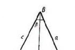
Imagine an isosceles triangle. This figure has one plane of symmetry perpendicular to the plane of the figure and passing through the perpendicular AO. For reflection, it is necessary from each point of the figure (for example, from the point IN) drop a perpendicular to the plane of symmetry OV and continue, this perpendicular for a distance equal to IN =B 1 O, and if the triangle is isosceles, then the reflection of the point IN aligned with point IN 1 , while the reflection is straight VA - with a straight line IN 1 A. The reflection of the left half is aligned with the right half. By doing the same with the right half of the figure, we will match its reflection with the left half, and as a result, the whole figure will be combined with itself. So, the figure will come to a new state, no different from the original.

In a cube, the shape of which crystals of most metals have, one can first of all find three mutually perpendicular symmetry planes, which, like the coordinate planes of an orthogonal system, bisect opposite parallel edges. Next, you can find the symmetry planes passing along the diagonals of the faces of the cube. As a result, there are 9 planes of symmetry in the cube, and they all intersect at one point - the center of the cube.

P
the simplest element of symmetry is a special point inside the figure - center of inversion (center of symmetry). For example, a point lying at the intersection of the diagonals of a parallelogram is characterized by the fact that any straight line drawn through it meets at equal distances from it the corresponding (identical) points of the parallelogram contour (for example, M And M 1 ). This singular point will be the center of symmetry. An example of a spatial figure, the symmetry of which is exhausted by the presence of one center of symmetry, is an oblique parallelepiped.

So, center of symmetry is called a special point inside the figure, characterized by the fact that on both sides of any line drawn through it and at equal distances from this line there are identical (corresponding) points of the figure. The considered symmetric transformation at the center of symmetry is a mirror reflection at a point.

Axis of symmetry is called a straight line belonging to a given figure, when rotated around it by some definite angle, the figure is combined with itself. This is possible if, firstly, the figure consists of several repeating equal parts and, secondly, these repeating equal parts are located in such a way that, when the figure is rotated through some well-defined angle, it will take the same position in space that it occupied before this turn. Only in this case, in place of some of its parts, other parts equal to them become. In this case, it is customary to say that the figure aligns with itself or self-combines.

Let's take some figure that has an axis of symmetry, for example, consisting of six equal triangles. According to the condition, the figure must be aligned with itself

P when rotated through some angle around the axis of symmetry. Obviously, the axis of symmetry runs perpendicular to the plane of the drawing through the center of the figure. The smallest angle of rotation at which the figure will self-align is 60 degrees, i.e. sixth of a complete revolution around the axis of symmetry. In this case, the figure under consideration will have only one element of symmetry - the axis.

The smallest angle through which a figure must be rotated around the axis of symmetry in order for the figure to align itself is called elementary angle of rotation given axis of symmetry. For the figure shown in this figure, it is 60 degrees.

The elementary angle of rotation of a given axis of symmetry determines the number of self-alignments of the figure when it is rotated around this axis by 360 degrees, or order axes of symmetry. If the elementary angle of rotation is denoted by A, and the order of the symmetry axis - through P, That n=360/a. It is proved that the orders of the symmetry axes can only be integers. The figure considered above, consisting of six equal triangles, has an axis of symmetry of the sixth order.

The axes of symmetry can be of any order. Through the center of a regular triangle, perpendicular to the plane of the drawing, a symmetry axis of the third order passes, through the center of a square - the fourth, through the center of a regular pentagon - the fifth, through the center of a regular hexagon - the sixth, and so on up to the circle, through the center of which passes the axis of symmetry of infinite order. The axes of a cone or cylinder are also the axes of symmetry of the infinite, just like any diameter of a sphere. Therefore, the ball has an infinite number of symmetry axes of infinite order.

Among the geometric figures, the form of which crystals can take, there are no figures with axes of the fifth order, as well as with axes of symmetry, the order of which is higher than the sixth. So, crystalline polyhedra have only axes of symmetry of 2-, 3-, 4- and 6-orders. The axis of the 2nd order is in the figure if the first self-alignment occurs when rotating around it 180 degrees. The axes of the 3rd, 4th, 6th orders correspond to the elementary angles of rotation by 120, 90, 60 degrees. In contrast to the dual axis, they are called higher order axes. A figure can have one or more axes of symmetry of the same or different orders.

The considered axes of symmetry are called simple. They are denoted by numbers indicating the order of the axis.

When writing a symmetry formula, which is a complete list of symmetry elements, use the letter L. The order of the axis of symmetry is indicated as a subscript letter L. (For example, the designations L h And L 4 correspond to the axes of symmetry of the 3rd and 4th orders.) The number of axes of symmetry of a given figure (crystal, texture, etc.) is indicated before L. (Let's say 4 L 3 should be interpreted as four axes of symmetry of the 3rd order.)

In addition to the considered simple operations that reveal symmetry in geometric shapes, other combined geometric transformations are possible, which consist of simultaneous rotation and reflection either at a point or in a plane. These complex geometric transformations are described using additional symmetry elements: inversion And mirror axes of symmetry.

mirror called the axis of symmetry, about which the figure rotates through an elementary angle, being simultaneously reflected in a plane perpendicular to it (this is not necessarily the plane of symmetry of the figure).

Inversion is the axis of symmetry, which, having the properties of a simple axis of symmetry of the same order, implies at the same time reflection at the point as the center of symmetry. The presence of a center of symmetry in a figure with an inversion axis of symmetry is also not necessary.

Inversion axes of symmetry are indicated by a number with a straight line, mirror ones with a wavy (tilde). For example, designations 3 and 4 correspond to the inversion and mirror axes of symmetry of the 3rd and 4th orders.

Symmetry groups

In addition to simple and complex symmetry elements that are present in geometric figures in a single number, there are well-defined sets of these symmetry elements, which are also observed in real figures. The complete set of symmetry elements of a geometric figure is called group(class, type) symmetry.

As a result of the derivation, 32 symmetry groups of crystalline polyhedra were obtained, and in addition to them, 5 symmetry groups of textured materials and 7 symmetry groups of rotation figures (see the table below).

There are several ways to describe the point symmetry groups of figures. Let's consider 2 of them:

1.B international In practice, the following designations are adopted: n - axis of symmetry n-th order (n = 2, 3, 4, ...);

- inversion axis n-th order (n = 1, 2, 3...);

T - plane of symmetry;

Fri - axis of symmetry n th order and a plane of symmetry passing along it ( 2t, 3t, 4t,...);

p/t - axis of symmetry of the nth order and the plane of symmetry perpendicular to it, as well as the center of symmetry for even axes (2/t, 3/t, 4/t,.)

p2 - axis of symmetry n-th order and P axes of the 2nd order, perpendicular to it (222, 322, 422, 522 , 622);

p/ttt- axis of symmetry n th order and plane T. parallel and perpendicular to it.

In international symbolism, only generative elements of symmetry are indicated in the symmetry class. Knowing the theorems on the combination of symmetry elements, it is possible to find the entire set of symmetry elements of a given class from the generating elements.

2.The table shows symmetry formulas- a set of elements for all kinds of symmetry. These formulas use symbolism of Bravais:

R - symmetry plane:

WITH- center of symmetry;

L i 1 , L i 2 , L i 3 ,... - inversion.

Each selected set of symmetry groups is characterized by the obligatory presence of certain elements.

A set of symmetry groups that have one or more similar elements is called syngony.

In crystallography, only seven syngonies are distinguished: triclinic. monoclinic, rhombic, trigonal, tetragonal, hexagonal and cubic. It is necessary to add the pentagonal system to the considered systems.

Symmetry of infinite figures

Consider an ideal crystal. In the structure of this crystal, which can be imagined as endless symmetrical rows, grids and lattices of periodically alternating particles, there are no violations: all identical particles are arranged in identical parallel rows. The distances between particles in most crystalline substances are several angstroms, therefore, even at a length of 1 mm, there are approximately 10 to the seventh power of particles in a crystal, which can practically be considered an infinite number.

The shortest possible distance between identical points in a series is called the shortest, or elementary, broadcast, or period of identity(rice. ...); names are sometimes used broadcast period, or row parameter.

If we shift the points of an infinite row by one period of identity along the direction of translation, then all identical points will move by the same distance, the row will coincide with itself, so that its view will not be disturbed. This is how it's made symmetrical transformation- the series is symmetrically shifted by one translation period A.

A translation, or a translation-assisted transformation, is a symmetric transformation by which a point is repeated in space.

P repeating any point using translation, we get an infinite periodic series of identical points at distances a, 2a, Za, ..., pa. The characteristic of this series is the shortest translation A. Identical points connected by translations A in an endless series are called knots row. The nodes do not have to coincide with the material particles of the substance, they can also be the same points between the particles of the substance.

Repeating the same points using another translation that is not parallel to the first one, we obtain a two-dimensional plane grid, which is completely defined by two elementary translations a andb or three arbitrary nodes that do not lie on one straight line. Parallelograms whose vertices are nodes are called cells grids. A flat grid can be defined by any pair of translations that do not lie on the same straight line (Fig. A). The choice of such a pair of basic parameters of a flat grid is not unambiguous, but it is customary to choose the shortest translations and precisely those that best reflect the symmetry of the grid.

We choose an elementary cell in a flat grid; repeating it using the same translations, we get a flat grid that fills the entire plane without gaps. The elementary cell can be chosen in different ways (Fig. b) but it is customary to choose it so that it satisfies the following conditions:

best reflected the symmetry of the grid;

if possible, it would have right angles;

would have the smallest area.

Primitive elementary cell a cell is called, inside which there are no nodes (Fig. V). Each node located at the top of such a cell belongs to four cells at the same time, which means that this cell accounts for only 1/4 of this node, and only one cell accounts for
node. The cell that contains one node can be chosen in different ways, but all the areas of such cells are the same regardless of the shape of the cell, because the area is a constant value for a given grid. The number of nodes per unit area is called reticular density grids.

Thus, a flat grid can be defined in three ways:

as a pair of elementary non-collinear translations, or

as a system of elementary nodes that can be obtained from one another using parallel transfers, or

as a system of identical elementary cells adjacent to each other, filling the plane without gaps and matching each other with the help of parallel transfers.

Two-dimensional symmetry groups can be obtained, as well as one-dimensional ones, by enumerating all combinations of admissible open and closed symmetry elements, then adding to each such combination the translational components of the corresponding flat grids. 17 two-dimensional symmetry groups are shown in the figure.

P
Let us now apply to an arbitrary point three elementary translations that do not lie in the same plane (non-coplanar) and repeat it infinitely in space. We get space grid, those. three-dimensional system of equivalent nodes.

ABOUT the main trio of broadcasts, the so-called translationalgroup, or a group of translations for a spatial lattice can be chosen in different ways, but it is customary to choose translations that are shortest and correspond to lattice symmetries.

Parallelepiped built on three elementary translations A,b,With, called elementary parallelepiped. or elementary cell. As in a flat grid, the volume of a primitive unit cell does not depend on its shape and is a constant value for a given grid; it is equal to the volume per node.

TO
Like a planar grid, a spatial grid can be defined in three ways:

as a trio of elementary non-coplanar translations, or

as a system of equivalent points that transform into each other using three basic translations, or

as a system of three identical parallelepipeds that densely fill the space and can be combined with each other using three main translations.

Any of these definitions gives the same scheme of the three-dimensional periodicity of the distribution of matter particles in a crystal.

For the edges of the elementary cell, i.e. for elementary translations, they take those directions in the spatial lattice in which the translation value is the smallest and which best reflect the symmetry of the lattice.

Based on the idea of ​​the periodic arrangement of the centers of gravity of spherical material particles in a crystalline substance, O. Bravais in 1848 showed that the entire variety of crystalline structures can be described using 14 types of lattices that differ in the shape of elementary cells and in symmetry and are divided into 7 crystals -

l graphic syngonies. These grids were named Bravais gratings.

Each Bravais lattice is broadcast group characterizing the arrangement of material particles in space.

Any crystalline

the structure can be represented using one of the 14 Bravais lattices.

To select a Bravais cell, 3 conditions are used:

1) the symmetry of the unit cell must correspond to the symmetry of the crystal, more precisely, the highest symmetry of the syngony to which the crystal belongs. Unit cell edges must be translations;

elementary cell must contain at most possible number right angles or equal angles and equal edges;

unit cell must have a minimum volume.

These conditions must be met sequentially, i.e. When choosing a cell, the first condition is more important than the second, and the second is more important than the third.

By the nature of the relative position of the main translations or by the location of the nodes, all crystal lattices are divided, according to Bravais, into 4 types:

primitive ( R),

base-centered ( C, B or A),

body-centered ( I),

face centered ( F).

In the primitive R In a cell, lattice nodes are located only at the vertices of the cell, and in complex cells there are more nodes. In a body-centered I- cell - one node in the center of the cell. in face-centered F-cell - one node in the center of each face. In base-centered WITH(A, B) - cell - one corner at the centers of a pair of parallel faces.

To isolate the elementary Bravais cell in the structure, it is necessary to find 3 shortest non-coplanar translations A,b, With, moreover, each translation must begin and end on the same nodes. Next, you need to check the basic requirements:

1) Is it possible to build a cell on these translations that meets the Bravais cell selection rules;

2) whether all particles in the structure can be obtained using such a set of translations.

In the general case, each syngony can correspond to lattices of all four types ( R, S,I, F), however, in fact, in all syngonies, except for the rhombic one, the number of possible Bravais lattices is reduced due to the reduction of some types of lattices to others. So, for example, in a cubic lattice: if a pair of faces of a cubic unit cell turns out to be centered, then, due to cubic symmetry, all other faces are centered, and instead of a base-centered one, a face-centered lattice is obtained.

The set of coordinates of the nodes included in the elementary cell is called basis cells. The entire crystal structure can be obtained by repeating the basis nodes of the set of translations of the Bravais cell. In this case, the origin of coordinates is chosen at the top of the cell and the coordinates of the nodes are expressed in fractions of elementary translations a, b, c.

The set of all symmetry operations of a crystal structure is called space symmetry group. The derivation of 230 space symmetry groups was completed by 1890 by the Russian crystallographer Evgraf Stepanovich Fedorov by 1891 by the German geometer Arthur Schoenflies. Fedorov was the first to arrive at the final results, so space groups are often called Fedorov's.

If, according to its external symmetry (macrosymmetry), each crystalline substance belongs to one of 32 classes, to one of 32 point groups, then the symmetry of its crystal structure (microsymmetry) corresponds to one of 230 space groups.

The existence of translations leads to the emergence of new symmetry elements, for example, glancing reflection plane(g). The amount of slip (advance) of the plane of grazing reflection is always equal to ½ translational vector coinciding with the direction of sliding, since a double reflection gives an equivalent point that is separated from the original one by the value of the whole translational vector.

Fractal Properties

Fractal properties are not a whim and not the fruit of an idle fantasy of mathematicians. By studying them, we learn to distinguish and predict important features objects and phenomena surrounding us, which before, if not completely ignored, were estimated only approximately, qualitatively, by eye. For example, by comparing the fractal dimensions of complex signals, encephalograms, or heart murmurs, doctors can diagnose some serious diseases at an early stage, when the patient can still be helped. Also, the analyst, comparing the previous behavior of prices, at the beginning of the formation of the model can foresee its further development, thereby avoiding gross errors in forecasting.

Irregularity of fractals

The first property of fractals is their irregularity. If a fractal is described by a function, then the property of irregularity in mathematical terms will mean that such a function is not differentiable, that is, not smooth at any point. Actually, this has the most direct relation to the market. Price fluctuations are sometimes so volatile and changeable that it confuses many traders. Our task is to sort out all this chaos and bring it to order.

Self-similarity of fractals

The second property says that a fractal is an object that has the property of self-similarity. This is a recursive model, each part of which repeats in its development the development of the entire model as a whole and is reproduced at various scales without visible changes. However, changes still occur, which can greatly affect our perception of the object.

Self-similarity means that the object does not have a characteristic scale: if it had such a scale, you would immediately distinguish the enlarged copy of the fragment from the original image. Self-similar objects have an infinite number of scales for all tastes. The essence of self-similarity can be explained by the following example. Imagine that you have a picture of a “real” geometric line, “length without width”, as Euclid defined the line, and you are playing with a friend, trying to guess whether he shows you the original picture (original) or a picture of any fragment of a straight line. No matter how hard you try, you will never be able to distinguish the original from the enlarged copy of the fragment, the straight line is arranged in the same way in all its parts, it is similar to itself, but this remarkable property of it is somewhat hidden by the uncomplicated structure of the straight line itself, its “straightness” (Fig. 35).

Rice. 35

If you also fail to distinguish a snapshot of some object from a properly enlarged snapshot of any of its fragments, then you have a self-similar object. All fractals that have at least some symmetry are self-similar. And this means that some fragments of their structure are strictly repeated at certain spatial intervals. Obviously, these objects can be of any nature, and their appearance and shape remain unchanged regardless of the scale. An example of a self-similar fractal:

Rice. 36

In finance, this concept is not a groundless abstraction, but a theoretical restatement of a practical market saying - namely, that the movements of a stock or a currency are superficially similar, regardless of the time frame and price. The observer cannot tell appearance graph, whether the data refers to weekly, daily or hourly changes.

Of course, not all fractals have such a regular, endlessly repeating structure as those wonderful exhibits of the future museum of fractal art, which were born from the imagination of mathematicians and artists. Many fractals found in nature (fault surfaces of rocks and metals, clouds, currency quotes, turbulent flows, foam, gels, soot particle contours, etc.) lack geometric similarity, but stubbornly reproduce in each fragment the statistical properties of the whole. Fractals with a non-linear form of development were named by Mandelbrot as multifractals. A multifractal is a quasi-fractal object with a variable fractal dimension. Naturally, real objects and processes are much better described by multifractals.

Such statistical self-similarity, or self-similarity on average, distinguishes fractals from a variety of natural objects.

Consider an example of self-similarity in the foreign exchange market:

Rice. 37

In these figures, we see that they are similar, while having a different time scale, in Fig. a minute scale, in Fig. b weekly price scale. As you can see, these quotes do not have the ability to perfectly repeat each other, however, we can consider them similar.

Even the simplest of fractals - geometrically self-similar fractals - have unusual properties. For example, a von Koch snowflake has a perimeter of infinite length, although it limits a finite area (Fig. 38). In addition, it is so prickly that it is impossible to draw a tangent to it at any point of the contour (a mathematician would say that a von Koch snowflake is nowhere differentiable, that is, not smooth at any point).

Rice. 38

Mandelbrot found that the results of fractional measurement remain constant for various degrees of enhancement of the object's irregularity. In other words, there is regularity (correctness, orderliness) for any irregularity. When we treat something as random, it indicates that we do not understand the nature of this randomness. In market terms, this means that the formation of the same typical formations must occur in different time frames. A one-minute chart will describe a fractal formation in the same way as a monthly one. Such "self-similarity", found on the charts of commodity and financial markets, shows all the signs that the market's actions are closer to the behavioral paradigm of "nature" than the behavior of economic, fundamental analysis.

Rice. 39

In these figures, you can find confirmation of the above. On the left is a graph with a minute scale, on the right is a weekly one. Here are the currency pairs Dollar/Yen (Fig. 39(a)) and Euro/Dollar (Fig. 39(b)) with different price scales. Even though the JPY/USD currency pair has a different volatility in relation to EUR/USD, we can observe the same price movement structure.

fractal dimension

The third property of fractals is that fractal objects have a dimension other than Euclidean (in other words, a topological dimension). The fractal dimension is a measure of the complexity of the curve. By analyzing the alternation of sections with different fractal dimensions and how the system is affected by external and internal factors, one can learn to predict the behavior of the system. And most importantly, to diagnose and predict unstable conditions.

In the arsenal of modern mathematics, Mandelbrot found a convenient quantitative measure of the imperfection of objects - the sinuosity of the contour, the wrinkling of the surface, the fracturing and porosity of the volume. It was proposed by two mathematicians - Felix Hausdorff (1868-1942) and Abram Samoylovich Besikovich (1891-1970). Now it deservedly bears the glorious names of its creators (Hausdorff-Besikovich dimension) - Hausdorff-Besikovich dimension. What is dimension and why do we need it in relation to the analysis of financial markets? Before that, we knew only one type of dimension - topological (Fig. 41). The word dimension itself indicates how many dimensions an object has. For a segment, a straight line, it is equal to 1, i.e. we have only one measurement, namely the length of a segment or a straight line. For a plane, the dimension will be 2, since we have a two-dimensional dimension, length and width. For space or solid objects, the dimension is 3: length, width, and height.

Let's take the example of computer games. If the game is made in 3D graphics, then it is spatial and voluminous, if in 2D graphics, the graphics are displayed on a plane (Fig. 40).

Rice. 40

Rice. 41

The most unusual (it would be more correct to say - unusual) in the dimension of Hausdorff - Besikovich was that it could take not only integers, as a topological dimension, but also fractional values. Equal to one for a straight line (infinite, semi-infinite or for a finite segment), the Hausdorff-Besikovich dimension increases as the tortuosity increases, while the topological dimension stubbornly ignores all changes that occur with the line.

Dimension characterizes the complication of a set (for example, a straight line). If this is a curve with a topological dimension equal to 1 (a straight line), then the curve can be complicated by an infinite number of bends and branches to such an extent that its fractal dimension approaches two, i.e. it fills almost the entire plane. (fig.42)

Rice. 42

By increasing its value, the Hausdorff-Besikovich dimension does not change it abruptly, as the topological dimension would do “in its place”, the transition from 1 immediately to 2. The Hausdorff-Besikovich dimension - and this at first glance may seem unusual and surprising, takes fractional values : equal to one for a straight line, it becomes 1.15 for a slightly sinuous line, 1.2 for a more sinuous line, 1.5 for a very sinuous line, and so on.

Rice. 43

It was in order to emphasize the ability of the Hausdorff-Besikovich dimension to take fractional, non-integer values ​​that Mandelbrot came up with his own neologism, calling it the fractal dimension. So, the fractal dimension (not only Hausdorff - Besikovich, but any other) - this is a dimension that can take not necessarily integer values, but also fractional ones.

For linear geometric fractals, the dimension characterizes their self-similarity. Consider Fig.48 (A), the line consists of N=4 segments, each of which has a length of r=1/3. As a result, we get the ratio:

D = logN/log(l/r)

The situation is quite different when we talk about multifractals (non-linear). Here the dimension loses its meaning as a definition of the similarity of an object and is defined through various generalizations, much less natural than the unique dimension of self-similar objects.

In the foreign exchange market, the dimension can characterize the volatility of price quotes. Each currency pair has its own behavior in terms of prices. For the Pound/Dollar pair (Fig. 44(a)) it is more calm than for the Euro/Dollar (Fig. 44(b)). The most interesting thing is that these currencies move with the same structure to price levels, however, they have different dimensions, which can affect intraday trading and changes in models that elude the inexperienced look.

Rice. 44

On fig. 45 shows the dimension in relation to the mathematical model, in order for you to more deeply penetrate into the meaning of this term. Note that all three figures show the same cycle. In fig.a the dimension is 1.2, in fig.b the dimension is 1.5, and in fig.c 1.9. It can be seen that with an increase in the dimension, the perception of the object becomes more complicated, the amplitude of oscillations increases.

Rice. 45

In financial markets, dimension is reflected not only as price volatility, but also as a detail of cycles (waves). Thanks to it, we will be able to distinguish whether a wave belongs to a certain time scale. Figure 46 shows the Euro/Dollar pair on a daily price scale. Pay attention, you can clearly see the formed cycle and the beginning of a new, larger cycle. By switching to an hourly scale and zooming in on one of the cycles, we can see smaller cycles, and part of a large one located at Dl(pHC.16). The detailing of cycles, i.e. their dimension, allows us to determine from the initial conditions how the situation can develop in the future. We can say that: fractal dimension reflects the property of scale invariance of the considered set.

The concept of invariance was introduced by Mandelbrot from the word "sealant" scalable, i.e. when an object has the property of invariance, it has different display scales.

Rice. 46

Rice. 47

In Fig. 47, circle A highlights a mini-cycle (detailed wave), circle B - a wave of a larger cycle. It is precisely because of the dimension that we cannot always determine ALL cycles on the same price scale.

We will talk about the problems of determining and developing properties of non-periodic cycles in the “Cycles in the foreign exchange market” section, now the main thing for us was to understand how and where dimension manifests itself in financial markets.

Thus, we can say that fractals as models are used when the real object cannot be represented in the form of classical models. And this means that we are dealing with non-linear relationships and the non-deterministic (random) nature of the data. Nonlinearity in the ideological sense means the multivariance of development paths, the availability of a choice from alternative paths and a certain pace of evolution, as well as the irreversibility of evolutionary processes. Nonlinearity in the mathematical sense means a certain type of mathematical equations (nonlinear differential equations) containing the desired quantities in powers greater than one or coefficients that depend on the properties of the medium. A simple example of a non-linear dynamical system:

Johnny grows 2 inches a year. This system explains how Johnny's height changes over time. Let x(n) be Johnny's height this year. Let his growth next year be written as x(n+1). Then we can write the dynamical system in the form of an equation:

x(n+1) = x(n)+2

See? Isn't this simple math? If we enter Johnny's height today x(n) = 38 inches, then on the right side of the equation we get Johnny's height next year, x(n+1) = 40 inches:

x(n+1) = x(n) + 2 = 38 + 2 = 40.

Moving from right to left in an equation is called iteration (repetition). We can repeat the equation again by inserting Johnny's new height of 40 inches on the correct side of the equation (i.e. x(n) = 40) and we get x(n+1) = 42. If we iterate (repeat) the equation 3 times, we we get Johnny's height in 3 years, namely 44 inches, starting with a height of 38 inches.

This is a deterministic dynamic system. If we want to make it non-deterministic (stochastic), we could make a model like this: Johnny grows 2 inches a year, more or less, and write the equation as:

x(n+1) = x(n) + 2 + e

where e is a small error (small relative to 2), represents some probability distribution.

Let's go back to the original deterministic equation. The original equation, x(n+1) = x(n) + 2, is linear. Linear means you are adding variables or constants, or multiplying variables by constants. For example, the equation

z(n+l) = z(n) + 5 y(n) -2 x(n)

is linear. But if you multiply the variables, or raise them to a power greater than one, the equation (system) will become non-linear. For example, the equation

x(n+1) = x(n)2

is non-linear because x(n) is squared. The equation

is non-linear because two variables, x and y, are multiplied.

When we apply classical models (for example, trend, regression, etc.), we say that the future of an object is uniquely determined, that is, it completely depends on the initial conditions and can be clearly predicted. You can independently perform one of these models in Excel. An example of a classical model can be represented as a constantly decreasing or increasing trend. And we can predict its behavior, knowing the past of the object (the initial data for modeling). And fractals are used in the case when the object has several options for development and the state of the system is determined by the position in which it is currently located. That is, we are trying to simulate a chaotic development. This system is the interbank foreign exchange market.

Let us now consider how one can obtain from a straight line what we call a fractal, with its inherent properties.

Figure 48 (A) shows the Koch curve. Let's take a line segment, its length = 1, that is, for the time being, the topological dimension. Now we will divide it into three parts (each 1/3 of the length), and remove the middle third. But we will replace the middle third with two segments (each 1/3 of the length), which can be represented as two sides of an equilateral triangle. This stage two (b) of the construction is depicted in Fig. 48 (A). At this point we have 4 smaller parts, each 1/3 of the length, so the whole length is 4(1/3) = 4/3. We then repeat this process for each of the 4 smaller lobes of the line. This is stage three (c). This will give us 16 even smaller line segments, each 1/9 of the length. So the whole length is now 16/9 or (4/3)2. As a result, we got a fractional dimension. But not only this distinguishes the resulting structure from a straight line. It has become self-similar and it is impossible to draw a tangent at any of its points (Fig. 48 (B))

Rice. 48

Application of fractals in the market

Given all of the above about fractals and their properties, we, working with a non-linear system of financial data, can apply them in our daily trading. And so let's look at the main advantages of fractals in the foreign exchange market:

1. The use of fractals will allow you to instantly remember almost the entire history of quotes of a currency pair. When will you remember a large number of price data, you will start to get a better feel for the trade. You will recognize patterns you never knew existed.

Why does the application of fractals give you this? Because by applying them, you bring chaos into order, and when the system is ordered in your head, you can easily find the item you need on the market, this is achieved using special exercises which will be described at the end of this course.

2. You will be able to analyze dozens of pairs, because now it will not be difficult for you. Using the properties of fractals will allow you to identify and navigate the market at a glance.

3. Applying the theory of fractals, you can not use other methods of analysis and make it unique in its kind.

4. Your outlook on the course of stock quotes will change. You won't wonder where am I? You will always have options.

5. You will begin to find situations on the chart SIMILAR to the course of currency prices at a given moment in time, which will allow you to prevent unreasonable losses and make a reliable forecast.

6. The theory of fractals is an abyss of ideas and their applications. By applying their properties to financial data, you can create your own unique trading system, which will include a combination of technical and fractal analysis.

7. You will look differently at the impact of news on the market.

8. And most importantly, now you will always have a card, without which you will no longer imagine yourself in the endless and alluring world of currencies.

Of course, I didn't list the whole list. positive sides the use of fractals in the market, you will already make the rest of the conclusions by yourself having studied this course to the end.

(Materials are based on: A. Almazov. Fractal theory. How to change your view of the markets)