The \(\chi^2\) test ("chi-square", also "Pearson's goodness-of-fit test") has an extremely wide application in statistics. In general terms, we can say that it is used to test the null hypothesis about the obedience of an observed random variable to a certain one. theoretical law distributions (see, for example, for details). The specific formulation of the hypothesis being tested will vary from case to case.
In this post, I will describe how the \(\chi^2\) test works using a (hypothetical) example from immunology. Imagine that we have performed an experiment to determine the effectiveness of suppressing the development of a microbial disease when the appropriate antibodies are introduced into the body. In total, 111 mice were involved in the experiment, which we divided into two groups, including 57 and 54 animals, respectively. The first group of mice was injected with pathogenic bacteria, followed by the introduction of blood serum containing antibodies against these bacteria. Animals from the second group served as controls - they received only bacterial injections. After some time of incubation, it turned out that 38 mice died, and 73 survived. Of the dead, 13 belonged to the first group, and 25 belonged to the second (control). The null hypothesis tested in this experiment can be formulated as follows: the administration of serum with antibodies has no effect on the survival of mice. In other words, we argue that the observed differences in the survival of mice (77.2% in the first group versus 53.7% in the second group) are completely random and are not associated with the action of antibodies.
The data obtained in the experiment can be presented in the form of a table:
Total |
|||
Bacteria + serum |
|||
Only bacteria |
|||
Total |
Tables like this one are called contingency tables. In this example, the table has a dimension of 2x2: there are two classes of objects ("Bacteria + serum" and "Bacteria only"), which are examined according to two criteria ("Dead" and "Survived"). This is the simplest case of a contingency table: of course, both the number of classes under study and the number of features can be larger.
To test the null hypothesis formulated above, we need to know what the situation would be if the antibodies did not really have any effect on the survival of mice. In other words, you need to calculate expected frequencies for the corresponding cells of the contingency table. How to do it? A total of 38 mice died in the experiment, which is 34.2% of the total number of animals involved. If the introduction of antibodies does not affect the survival of mice, the same percentage of mortality should be observed in both experimental groups, namely 34.2%. Calculating how much is 34.2% of 57 and 54, we get 19.5 and 18.5. These are the expected mortality rates in our experimental groups. The expected survival rates are calculated in a similar way: since 73 mice survived in total, or 65.8% of their total number, the expected survival rates are 37.5 and 35.5. Let's make a new contingency table, now with the expected frequencies:
dead |
Survivors |
Total |
|
Bacteria + serum |
|||
Only bacteria |
|||
Total |
As you can see, the expected frequencies are quite different from the observed ones, i.e. administration of antibodies does seem to have an effect on the survival of mice infected with the pathogen. We can quantify this impression using Pearson's goodness-of-fit test \(\chi^2\):
\[\chi^2 = \sum_()\frac((f_o - f_e)^2)(f_e),\]
where \(f_o\) and \(f_e\) are the observed and expected frequencies, respectively. The summation is performed over all cells of the table. So, for the example under consideration, we have
\[\chi^2 = (13 – 19.5)^2/19.5 + (44 – 37.5)^2/37.5 + (25 – 18.5)^2/18.5 + (29 – 35.5)^2/35.5 = \]
Is \(\chi^2\) large enough to reject the null hypothesis? To answer this question, it is necessary to find the corresponding critical value of the criterion. The number of degrees of freedom for \(\chi^2\) is calculated as \(df = (R - 1)(C - 1)\), where \(R\) and \(C\) are the number of rows and columns in the table conjugacy. In our case \(df = (2 -1)(2 - 1) = 1\). Knowing the number of degrees of freedom, we can now easily find out the critical value \(\chi^2\) using the standard R-function qchisq() :
Thus, for one degree of freedom, the value of the criterion \(\chi^2\) exceeds 3.841 only in 5% of cases. The value we obtained, 6.79, significantly exceeds this critical value, which gives us the right to reject the null hypothesis that there is no relationship between the administration of antibodies and the survival of infected mice. Rejecting this hypothesis, we risk being wrong with a probability of less than 5%.
It should be noted that the above formula for the criterion \(\chi^2\) gives somewhat overestimated values when working with contingency tables of size 2x2. The reason is that the distribution of the \(\chi^2\) criterion itself is continuous, while the frequencies of binary features ("died" / "survived") are discrete by definition. In this regard, when calculating the criterion, it is customary to introduce the so-called. continuity correction, or Yates amendment :
\[\chi^2_Y = \sum_()\frac((|f_o - f_e| - 0.5)^2)(f_e).\]
Pearson "s Chi-squared test with Yates" continuity correction data : mice X-squared = 5.7923 , df = 1 , p-value = 0.0161
As you can see, R automatically applies the Yates correction for continuity ( Pearson's Chi-squared test with Yates' continuity correction). The value \(\chi^2\) calculated by the program was 5.79213. We can reject the null hypothesis of no antibody effect at the risk of being wrong with a probability of just over 1% (p-value = 0.0161 ).
The chi-square distribution is one of the most widely used in statistics for testing statistical hypotheses. On the basis of the "chi-square" distribution, one of the most powerful goodness-of-fit tests, Pearson's "chi-square" test, was constructed.
The goodness-of-fit test is a criterion for testing the hypothesis about the proposed law of the unknown distribution.
The χ2 ("chi-square") test is used to test the hypothesis of different distributions. This is his merit.
The calculation formula of the criterion is equal to
where m and m' are the empirical and theoretical frequencies, respectively
distribution under consideration;
n is the number of degrees of freedom.
For verification, we need to compare empirical (observed) and theoretical (calculated under the assumption normal distribution) frequency.
If the empirical frequencies completely coincide with the frequencies calculated or expected, S (E - T) = 0 and the criterion χ2 will also be zero. If S (E - T) is not equal to zero, this will indicate a discrepancy between the calculated frequencies and the empirical frequencies of the series. In such cases, it is necessary to evaluate the significance of the χ2 criterion, which theoretically can vary from zero to infinity. This is done by comparing the actually obtained value of χ2ph with its critical value (χ2st). accepted level significance (a) and number of degrees of freedom (n).
The distribution of probable values of the random variable χ2 is continuous and asymmetric. It depends on the number of degrees of freedom (n) and approaches a normal distribution as the number of observations increases. Therefore, the application of the χ2 criterion to the estimate discrete distributions is associated with some errors that affect its value, especially for small samples. To obtain more accurate estimates, the sample distributed in variation series, must have at least 50 options. The correct application of the χ2 criterion also requires that the frequencies of variants in the extreme classes should not be less than 5; if there are less than 5 of them, then they are combined with the frequencies of neighboring classes so that their total amount is greater than or equal to 5. According to the combination of frequencies, the number of classes (N) also decreases. The number of degrees of freedom is set according to the secondary number of classes, taking into account the number of restrictions on the freedom of variation.
Since the accuracy of determining the criterion χ2 largely depends on the accuracy of calculating the theoretical frequencies (T), unrounded theoretical frequencies should be used to obtain the difference between the empirical and calculated frequencies.
As an example, take a study published on a website dedicated to the application statistical methods in the humanities.
The Chi-square test allows comparison of frequency distributions, whether they are normally distributed or not.
Frequency refers to the number of occurrences of an event. Usually, the frequency of occurrence of an event is dealt with when the variables are measured in the scale of names and their other characteristics, except for the frequency, are impossible or problematic to select. In other words, when the variable has qualitative characteristics. Also, many researchers tend to translate test scores into levels (high, medium, low) and build tables of score distributions to find out the number of people at these levels. To prove that in one of the levels (in one of the categories) the number of people is really more (less), the Chi-square coefficient is also used.
Let's take a look at the simplest example.
A self-esteem test was conducted among younger adolescents. Test scores were translated into three levels: high, medium, low. The frequencies were distributed as follows:
High (H) 27 pers.
Medium (C) 12 people
Low (H) 11 pers.
Obviously, children with high self-esteem majority, but this needs to be statistically proven. To do this, we use the Chi-square test.
Our task is to check whether the obtained empirical data differ from the theoretically equally probable ones. To do this, it is necessary to find the theoretical frequencies. In our case, theoretical frequencies are equiprobable frequencies that are found by adding all frequencies and dividing by the number of categories.
In our case:
(B + C + H) / 3 \u003d (27 + 12 + 11) / 3 \u003d 16.6
The formula for calculating the chi-square test is:
χ2 = ∑(E - T)І / T
We build a table:
Find the sum of the last column:
Now you need to find the critical value of the criterion according to the table of critical values (Table 1 in the Appendix). To do this, we need the number of degrees of freedom (n).
n = (R - 1) * (C - 1)
where R is the number of rows in the table, C is the number of columns.
In our case, there is only one column (meaning the original empirical frequencies) and three rows (categories), so the formula changes - we exclude the columns.
n = (R - 1) = 3-1 = 2
For the error probability p≤0.05 and n = 2, the critical value χ2 = 5.99.
The empirical value obtained is greater than the critical value - the frequency differences are significant (χ2= 9.64; p≤0.05).
As you can see, the calculation of the criterion is very simple and does not take much time. The practical value of the chi-square test is enormous. This method is most valuable in the analysis of responses to questionnaires.
Let's take a more complex example.
For example, a psychologist wants to know if it is true that teachers are more biased towards boys than towards girls. Those. more likely to praise girls. To do this, the psychologist analyzed the characteristics of the students written by the teachers for the frequency of occurrence of three words: "active", "diligent", "disciplined", the synonyms of the words were also counted. Data on the frequency of occurrence of words were entered in the table:
To process the obtained data, we use the chi-square test.
To do this, we construct a table of distribution of empirical frequencies, i.e. the frequencies that we observe:
Theoretically, we expect the frequencies to be distributed equally, i.e. the frequency will be distributed proportionally between boys and girls. Let's build a table of theoretical frequencies. To do this, multiply the row sum by the column sum and divide the resulting number by the total sum (s).
The resulting table for calculations will look like this:
χ2 = ∑(E - T)І / T
n = (R - 1), where R is the number of rows in the table.
In our case, chi-square = 4.21; n = 2.
According to the table of critical values of the criterion, we find: at n = 2 and an error level of 0.05, the critical value χ2 = 5.99.
The resulting value is less than the critical value, which means that the null hypothesis is accepted.
Conclusion: teachers do not attach importance to the gender of the child when writing his characteristics.
Conclusion.
K. Pearson made a significant contribution to the development of mathematical statistics ( a large number of fundamental concepts). Pearson's main philosophical position is formulated as follows: the concepts of science are artificial constructions, means of describing and ordering sensory experience; the rules for linking them into scientific proposals are singled out by the grammar of science, which is the philosophy of science. To connect heterogeneous concepts and phenomena allows a universal discipline - applied statistics, although according to Pearson it is also subjective.
Many constructions of K. Pearson are directly related or developed using anthropological materials. He developed numerous methods of numerical classification and statistical criteria used in all fields of science.
Literature.
1. A. N. Bogolyubov, Mathematics. Mechanics. Biographical guide. - Kyiv: Naukova Dumka, 1983.
2. Kolmogorov A. N., Yushkevich A. P. (ed.). Mathematics of the 19th century. - M.: Science. - T.I.
3. 3. Borovkov A.A. Math statistics. Moscow: Nauka, 1994.
4. 8. Feller V. Introduction to the theory of probability and its applications. - M.: Mir, T.2, 1984.
5. 9. Harman G., Modern factorial analysis. - M.: Statistics, 1972.
The quantitative study of biological phenomena necessarily requires the creation of hypotheses that can be used to explain these phenomena. To test this or that hypothesis, a series of special experiments is put in place and the actual data obtained are compared with those theoretically expected according to this hypothesis. If there is a match, this may be sufficient reason to accept the hypothesis. If the experimental data are in poor agreement with the theoretically expected, there is great doubt about the correctness of the proposed hypothesis.
The degree of compliance of the actual data with the expected (hypothetical) is measured by the chi-square fit test:
the actually observed value of the feature in i- toy; - the theoretically expected number or sign (indicator) for a given group, k-number of data groups.
The criterion was proposed by K. Pearson in 1900 and is sometimes called Pearson's criterion.
Task. Among 164 children who inherited the factor from one parent and the factor from the other, there were 46 children with the factor, 50 with the factor, 68 with both. Calculate expected frequencies at a 1:2:1 ratio between groups and determine the degree of agreement between empirical data using Pearson's test.
Solution: The ratio of observed frequencies is 46:68:50, theoretically expected 41:82:41.
Let's set the significance level to 0.05. The tabular value of the Pearson test for this level of significance with the number of degrees of freedom equal to it turned out to be 5.99. Therefore, the hypothesis about the correspondence of the experimental data to the theoretical one can be accepted, since, .
Note that when calculating the chi-square test, we no longer set the condition for the indispensable normality of the distribution. The chi-square test can be used for any distributions that we are free to choose in our assumptions. There is some universality in this criterion.
Another application of Pearson's criterion is the comparison of an empirical distribution with a Gaussian normal distribution. At the same time, it can be attributed to the group of criteria for checking the normality of the distribution. The only restriction is the fact that the total number of values (variant) when using this criterion must be large enough (at least 40), and the number of values in individual classes (intervals) must be at least 5. Otherwise, adjacent intervals should be combined. The number of degrees of freedom when checking the normality of the distribution should be calculated as:.
Fisher's criterion.
This parametric test serves to test the null hypothesis about the equality of the variances of normally distributed populations.
![]() Or.
Or.
For small sample sizes, the application of the Student's t-test can be correct only if the variances are equal. Therefore, before testing the equality of sample means, it is necessary to make sure that the Student's t-test is valid.
Where N 1 , N 2 sample sizes, 1 , 2 - the number of degrees of freedom for these samples.
When using tables, it should be noted that the number of degrees of freedom for a sample with a larger variance is chosen as the column number of the table, and for a smaller variance, as the row number of the table.
For the significance level according to the tables of mathematical statistics, we find a tabular value. If, then the hypothesis of equality of variances is rejected for the chosen level of significance.
Example. Studied the effect of cobalt on the body weight of rabbits. The experiment was carried out on two groups of animals: experimental and control. Experienced received an additive to the diet in the form of an aqueous solution of cobalt chloride. During the experiment, weight gain was in grams:
|
Control |
|

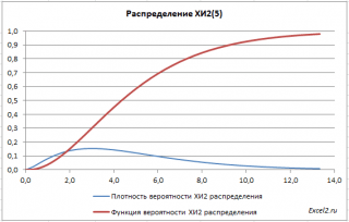
Consider the chi-squared distribution. Using the MS EXCEL functionCHI2.DIST() we will construct graphs of the distribution function and probability density, we will explain the application of this distribution for the purposes of mathematical statistics.
Chi-square distribution (X 2, XI2, EnglishChi- squareddistribution) applied in various methods mathematical statistics:
- when building;
- at ;
- at (whether the empirical data is consistent with our assumption about the theoretical distribution function or not, eng. Goodness-of-fit)
- at (used to determine the relationship between two categorical variables, eng. Chi-square test of association).
Definition: If x 1 , x 2 , …, x n are independent random variables distributed over N(0;1), then the distribution of the random variable Y=x 1 2 + x 2 2 +…+ x n 2 has distribution X 2 with n degrees of freedom.
Distribution X 2 depends on a single parameter called degree of freedom (df, degreesoffreedom). For example, when building number of degrees of freedom is equal to df=n-1, where n is the size samples.
Distribution density X 2
expressed by the formula:
Function Graphs
Distribution X 2 has an asymmetric shape, equal to n, equal to 2n.
IN example file on sheet Graph given distribution density plots probabilities and integral distribution function.
Useful property chi2 distributions
Let x 1 , x 2 , …, x n be independent random variables distributed over normal law with the same parameters μ and σ, and X cf is arithmetic mean these values x.
Then random value y equal
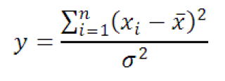
It has X 2 -distribution with n-1 degrees of freedom. Using the definition, the above expression can be rewritten as follows:

Hence, sampling distribution statistics y, with sampling from normal distribution, It has X 2 -distribution with n-1 degrees of freedom.
We will need this property for . Because dispersion can only be positive number, A X 2 -distribution used to evaluate it y d.b. >0, as stated in the definition.
HI2 distribution in MS EXCEL
In MS EXCEL, starting from version 2010, for X 2 -distributions there is a special function XI2.DIST() , English name– CHISQ.DIST(), which allows you to calculate probability density(see formula above) and (probability that a random variable X having XI2-distribution, takes a value less than or equal to x, P(X<= x}).
Note: Because chi2 distribution is a special case, then the formula =GAMMA.DIST(x,n/2,2,TRUE) for a positive integer n returns the same result as the formula =XI2.DIST(x, n, TRUE) or =1-XI2.DIST.X(x;n) . And the formula =GAMMA.DIST(x,n/2,2,FALSE) returns the same result as the formula =XI2.DIST(x, n, FALSE), i.e. probability density XI2 distributions.
The CH2.DIST.RT() function returns distribution function, more precisely, the right-handed probability, i.e. P(X > x). It is obvious that the equality
=CHI2.DIST.X(x;n)+ CHI2.DIST(x;n;TRUE)=1
because the first term calculates the probability P(X > x), and the second P(X<= x}.
Prior to MS EXCEL 2010, EXCEL had only the HI2DIST() function, which allows you to calculate the right-hand probability, i.e. P(X > x). The capabilities of the new MS EXCEL 2010 functions CHI2.DIST() and CHI2.DIST.RT() overlap the capabilities of this function. The HI2DIST() function was left in MS EXCEL 2010 for compatibility.
CHI2.DIST() is the only function that returns probability density of the chi2 distribution(third argument must be FALSE). The rest of the functions return integral distribution function, i.e. the probability that a random variable will take a value from the specified range: P(X<= x}.
The above functions of MS EXCEL are given in.
Examples
Find the probability that the random variable X will take a value less than or equal to the given x: P(X<= x}. Это можно сделать несколькими функциями:
CHI2.DIST(x, n, TRUE)
=1-CHI2.DIST.RP(x; n)
=1-CHI2DIST(x; n)
The function XI2.DIST.X() returns the probability P(X > x), the so-called right-handed probability, so to find P(X<= x}, необходимо вычесть ее результат от 1.
Let's find the probability that the random variable X will take on a value greater than the given one x: P(X > x). This can be done with several functions:
1-CHI2.DIST(x, n, TRUE)
=XI2.DIST.RP(x; n)
=CHI2DIST(x, n)
Inverse chi2 distribution function
The inverse function is used to calculate alpha- , i.e. to calculate values x for a given probability alpha, and X must satisfy the expression P(X<= x}=alpha.
The CH2.INV() function is used to calculate confidence intervals of the normal distribution variance.
The XI2.INV.RT() function is used to calculate , i.e. if a significance level is specified as an argument of the function, for example, 0.05, then the function will return such a value of the random variable x, for which P(X>x)=0.05. As a comparison: the function XI2.INV() will return such a value of the random variable x, for which P(X<=x}=0,05.
In MS EXCEL 2007 and earlier, instead of XI2.OBR.RT(), the XI2OBR() function was used.
The above functions can be interchanged, as the following formulas return the same result:
=CHI.OBR(alpha,n)
=XI2.INV.RT(1-alpha;n)
\u003d XI2OBR (1-alpha; n)
Some calculation examples are given in example file on the Functions sheet.
MS EXCEL functions using the chi2 distribution
Below is the correspondence between Russian and English function names:
HI2.DIST.PH() - eng. name CHISQ.DIST.RT, i.e. CHI-SQuared DISTribution Right Tail, the right-tailed Chi-square(d) distribution
XI2.OBR () - English. name CHISQ.INV, i.e. CHI-Squared distribution INVerse
HI2.PH.OBR() - English. name CHISQ.INV.RT, i.e. CHI-SQuared distribution INVerse Right Tail
HI2DIST() - eng. name CHIDIST, function equivalent to CHISQ.DIST.RT
HI2OBR() - eng. the name CHIINV, i.e. CHI-Squared distribution INVerse
Estimation of distribution parameters
Because usually chi2 distribution used for the purposes of mathematical statistics (calculation confidence intervals, hypothesis testing, etc.) and almost never for constructing models of real values, then for this distribution, the discussion of estimating the distribution parameters is not carried out here.
Approximation of the XI2 distribution by the normal distribution
With the number of degrees of freedom n>30 distribution X 2 well approximated normal distribution co averageμ=n and dispersion σ=2*n (see example file sheet Approximation).
Pearson distributions (chi - square), Student and Fisher
The normal distribution defines three distributions that are now commonly used in statistical data processing. In the following sections of the book, these distributions are encountered many times.
Pearson distribution (chi - square) - distribution of a random variable
where random variables X 1 , X 2 ,…, X n are independent and have the same distribution N(0.1). In this case, the number of terms, i.e. n, is called the "number of degrees of freedom" of the chi-squared distribution.
The chi-square distribution is used in estimating variance (using a confidence interval), in testing hypotheses of agreement, homogeneity, independence, primarily for qualitative (categorized) variables that take on a finite number of values, and in many other tasks of statistical data analysis.
Distribution t Student is the distribution of a random variable
where random variables U And X independent, U has a standard normal distribution N(0,1) and X– distribution chi – square with n degrees of freedom. Wherein n is called the "number of degrees of freedom" of the Student's distribution.
Student's distribution was introduced in 1908 by the English statistician W. Gosset, who worked at a beer factory. Probabilistic-statistical methods were used to make economic and technical decisions at this factory, so its management forbade V. Gosset to publish scientific articles under his own name. In this way, a trade secret was protected, "know-how" in the form of probabilistic-statistical methods developed by W. Gosset. However, he was able to publish under the pseudonym "Student". The history of Gosset-Student shows that a hundred years ago, the great economic efficiency of probabilistic-statistical methods was obvious to British managers.
Currently, the Student's distribution is one of the most well-known distributions among those used in the analysis of real data. It is used in estimating the mathematical expectation, predictive value and other characteristics using confidence intervals, testing hypotheses about the values of mathematical expectations, regression coefficients, hypotheses of sample homogeneity, etc. .
The Fisher distribution is the distribution of a random variable
where random variables X 1 And X 2 are independent and have chi distributions - the square with the number of degrees of freedom k 1 And k 2 respectively. At the same time, a couple (k 1 , k 2 ) is a pair of "numbers of degrees of freedom" of the Fisher distribution, namely, k 1 is the number of degrees of freedom of the numerator, and k 2 is the number of degrees of freedom of the denominator. Distribution of a random variable F named after the great English statistician R. Fisher (1890-1962), who actively used it in his work.
The Fisher distribution is used to test hypotheses about the adequacy of the model in regression analysis, about the equality of variances, and in other problems of applied statistics.
Expressions for the chi-square, Student and Fisher distribution functions, their densities and characteristics, as well as the tables necessary for their practical use, can be found in the specialized literature (see, for example,).