Numerical schemes for solving hyperbolic equations. Numerical Methods for Solving Partial Differential Equations of Hyperbolic Type (on the Example of the Transport Equation)

Consider the Cauchy problem for an equation of the form

in which the transfer rate v could be a function X. For equation (6.1), one can propose a set of difference schemes that differ in the order of approximation, the way in which derivatives are represented, and so on. Let us first dwell on explicit difference schemes, in which each equation of the system contains only one unknown quantity)", which makes it possible to sequentially calculate the values ​​of the solution on a new time layer.

It is known that the most important property, which explicit difference schemes must have, is the stability - the ability of the scheme not to accumulate computational perturbations. The stability of the scheme is a necessary requirement to ensure the convergence of the difference solution to the exact one. For a hyperbolic equation, stability analysis is usually carried out with respect to initial data based on the spectrum of eigenvalues ​​of the transition operator to a new time layer, based on which difference schemes acceptable for calculations are selected. Thus, the symmetric difference scheme

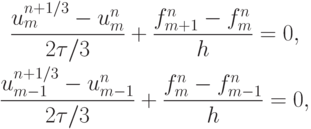
has a very strict stability condition (t 2 vh) and is not used for practical algorithms. Difference schemes

are conditionally stable. To ensure their stability, it is necessary, first, to fulfill the Courant Friedrichs-Levy (CFL) condition:

and secondly, the use of differences against the flow, i.e. application of scheme (6.3) for V> 0 and (6.4) for v0.

Explicit scheme with differences against the flow. If we selectively apply the two previous schemes, namely, with v >> 0 scheme (6.3), and for v

will be indifferent to the direction of speed and stable under the condition v/h^ 1. It is easy to see that one-sided differences in this scheme are taken towards the flow (it is said that the scheme has the property mpanenopmuenoemu). Schemes)" of this type are called upwind or scheme with differences against the flow.

In the case of an equation with constant value there are no problems with the design of the upwind difference scheme. The difference corresponding to the sign of the transfer rate is selected, which is used in all nodes of the computational domain. Condition (6.5) imposes a constraint on the ratio of computational grid steps. Usually, for a given space step, relation (6.5) determines the admissible time step m h/v.

But if the transfer rate is a function of the coordinate (or time), then the choice of the type of difference approximation must be carried out based on the analysis of the sign of the transfer rate, for example, using a conditional operator. Except goth, with variable transfer speed v = v(x) the stability condition must be checked for all grid nodes and from this set of time step values, the minimum must be chosen: t min,; h/vj.

Courant et al. (1952) proposed an interesting method for constructing an upwind scheme that did not use a conditional operator. It is important to note that this is not just a formal technique, but an approach containing deep ideas, on the basis of which one can compare and find a correspondence between upwind (asymmetric) and symmetric difference schemes. The idea of ​​splitting operators of difference schemes is close to this.

We represent the transfer rate as the sum of its positive and negative components:

This will allow the transfer operator to be represented as the sum of two operators:

Now each of the operators has a coefficient of constant sign, which makes it possible to apply the upwind difference approximation to it. Note that the counterflow difference scheme for approximating convective terms is widely used in various problems of computational fluid dynamics. The following notation of the computational algorithm according to the scheme (6.6) is often used:

If we now carry out elementary transformations on the right-hand side of (6.7) and single out the symmetric difference derivative, then this scheme can be represented as

It can be concluded that the upwind difference scheme (6.7) is equivalent to the symmetric one (6.2), which has a dissipative additive that ensures the conditional stability of the scheme.

Lax's scheme. This scheme was introduced into the practice of computing at the dawn of the development of computational gas dynamics. II although this type of scheme was mentioned in the works of various authors, public opinion associates it with the name of the American mathematician Lax (Lax, P.D.), who published a series of papers on various aspects of the theory of difference schemes in the 1950s. As applied to the transport equation (6.1), this scheme has the form

A feature of the scheme is that to ensure its stability in the approximation of the time derivative, the value of the grid function at the node (r, P) is replaced by the half-sum of the values ​​at neighboring nodes of the same time layer. This operation ensures the conditional stability of the difference scheme under the central approximation of the spatial derivative (when the Courant-Friedrichs-Levy condition is satisfied v/h ^ 1).

Although here the derivative with respect to X is presented with the second order of approximation, the scheme has significant dissipation due to the specific representation of the time derivative. This is clearly seen from the first differential approximation:

The coefficient on the right side in front of the second derivative can be interpreted as the scheme viscosity coefficient. After simple transformations, this quantity can be represented as

where through A denoted by the Courant number. Many properties of this scheme can be determined from the differential approximation:

• - the scheme becomes non-dissipative when the Courant number is equal to one;
• - the scheme is not sensitive to the flow direction;

when the Courant number is less than one, the circuit viscosity has a stabilizing effect (positive diffusion coefficient), when the Courant number is greater than one, the circuit viscosity coefficient becomes negative, which leads to an aggravation of the diffusion process and, ultimately, to the loss of computational stability of the circuit;

As the time step decreases, the dissipative properties of the scheme increase.

Among these features, there are those that significantly reduce the advantages of the scheme. However, the simplicity of the algorithm is often the basis for its use at the initial (debugging) steps of constructing computational programs. In addition, the Lax scheme, as we will see below, is integral part efficient multi-step algorithms, in which a preliminary step (prediction step) is performed with its help.

Schemes of the second order. The difference schemes discussed earlier were first-order schemes (with respect to the spatial or temporal variable). When constructing second-order schemes, it is necessary to provide an increased order of approximation both in terms of spatial and temporal variables. Consider several schemes of this type.

Leapfrog scheme. The second-order scheme, both in the space variable and in time, of the simplest type can be represented as

This circuit is called the stepping circuit, but it is better known as "leapfrog"(leap-frog scheme). The scheme is three-layered and builds a solution from the two previous time layers. Therefore, when using it, problems arise with the start of calculations, which should be carried out by some other method.

Lax-Wendroff scheme. One of the most famous schemes of this type is central circuit, called by the name of its authors, the Lax-Wendroff scheme. It has occupied a certain niche in the theory of difference schemes for hyperbolic equations, many very productive ideas are associated with it, but its main advantage is that it can be easily generalized and transferred to the case of more complex problems - problems of compressible gas flow described by systems of quasilinear equations, where it has been one of the main computing tools for quite a long time.

It is useful to study the features of this scheme by the example of its application to a transport equation of the form (6.1). To construct a second-order scheme, we write the Taylor formula:

which we will consider together with the original equation (6.1) This equation will be used to replace the time derivatives in the expansion with spatial ones. This is possible, since the first time derivative is expressed directly from (6.1): du/dt = -vdu/dx. The second derivative is also easily found from the following chain of relations:

Note that this representation is accurate only at a constant transfer rate: v= const. Otherwise, it is approximate, however, if the transfer rate v(x) is a sufficiently smooth function, it can be used for transformations of difference relations that are local in nature.

Substituting the expressions for the derivatives obtained using the original differential equation into the above Taylor formula, we obtain the relation

and replacing the space derivatives with second-order finite-difference relations, we obtain (after some simple transformations) the difference scheme

called the Lax Wendroff scheme. This scheme was introduced into the practice of computing along with a number of others in a series of papers published by Laks and Vsndroff in 1960-1964.

A two-step version of the Lax-Wendroff scheme. Later, Richtmeier proposed an original two-step version of the scheme, which, due to its ease of implementation, was one of the main computational algorithms in gas dynamics for a long time. Let's take this option.

At the first half-step, we calculate the intermediate value of the solution using a simple first-order Lax scheme. We assign a superscript to this intermediate value n+ 1/2 and keep in mind that the half time step is also used. Applying this scheme, we obtain the values ​​of the solution on the intermediate time layer: t = tn+l / 2 . Note that due to the use of the Lax scheme, in which there is no central node on the lower layer, the solution is also reproduced on the intermediate layer in the system of half-integer points.

Let us write down the difference relations for two neighboring gaps:

The second half step is to calculate the solution on a new time layer P+ 1 based on a scheme with central differences both in space and time - the "cross" scheme. To calculate the spatial derivatives, the values ​​of the solution on the intermediate layer in the system of half-integer points are used, the solution itself is restored in the same system of points in which it was determined by the beginning of the time step:

Relations (6.12) and (6.13) together determine the two-step Lax-Weidroff scheme. At its first stage, the stability conditions are satisfied. This stage is sometimes called predictor. The second stage ensures that the required accuracy is met and is called corrector. Predictor-corrector methods are often used in computational mathematics, and the corrector stage may include an iterative block.

It can be easily shown that, excluding intermediate values ​​from (6.13), with the help of relations (6.12) we arrive at the basic one-step version of the scheme. In terms of the order of approximation and stability, both options are equivalent, but the two-step one is more convenient for calculations, so the name of this difference scheme is usually associated with it. The two-step version is especially convenient to use when constructing difference schemes for more complex problems, in particular, for systems of quasilinear equations of nonstationary gas dynamics.

Monotonicity of the solution in second-order schemes. The last term on the right-hand side of (6.11) has a form different from that of the dissipative terms of the first-order schemes (6.8) and (6.10). In this case, it provides suppression of the error associated with the first order approximation of the time derivative. Thus, this scheme is a scheme of the second order in both time and space. Its first differential approximation will no longer contain a dissipative term, but it will contain a dispersion component with a third derivative, which is the cause of phase errors in the circuit. It can be expected that this scheme will slightly smear the solution, but nonphysical oscillations caused by dispersion may appear in the region of its sharp change.

A difference scheme that converts a solution that has the form of a monotonic function of the longitudinal coordinate into a monotonic solution is called monotone difference scheme. According to this definition, the Lax-Weidroff scheme is nonmonotonic.

S.K. Godunov established the monotonicity theorem, which occupies one of the central places in the theory of difference schemes. According to this theorem, for a linear equation of the form (6.1), there are no monotone schemes with an order greater than the first.

The loss of monotonicity of the difference scheme is typical to some extent for all schemes of higher approximation order. To overcome the nonmonotonicity of the numerical solution of the schemes high order use the so-called hybrid difference schemes. They belong to the class of non-linear ones, in which, based on the analysis of the behavior of the solution, they switch to monotonic first-order schemes in areas where phase errors are especially pronounced, and return to high-order schemes in areas of smooth change in the solution.

McCormack's scheme. It is also a two-step second-order scheme, indifferent to the flow direction. It is more convenient to demonstrate it in the conservative form of the transport equation:

The scheme consists of two successive steps:

At the first stage (6.15) find the preliminary value of the solution sch at the grid nodes based on a one-sided difference scheme. According to the solution found in this way, preliminary values ​​of the flows /r are calculated. Further, on the basis of one-way schemes having the opposite direction (6.16), the solution is determined at the next time layer.

This algorithm allows various modifications; it adapts well to solving both quasilinear systems and multidimensional hyperbolic problems. In the 1970s, this scheme was one of the main difference schemes of foreign (mainly American) calculators, but at present it has been superseded by more modern ones based on the ideas of hybridization.

Let us now consider the simplest difference schemes for the Hopf equation.

The generalization of the P. Lax scheme to the case of the Hopf equation has the form

Here, obviously, the divergent form of Eq. (3.6) is used.

Exercises. Consider the Lax-Wendroff scheme for the Hopf equation. Let the initial conditions for the Cauchy problem be set as follows: u(x, 0) = ch - 2 (x) . Then the Hopf equation has a first integral: . Check that the above schema is conservative, i.e. in it, the same conservation law is automatically satisfied at the grid level.

Build a similar circuit using characteristic form writing the Hopf equation (3.9). Will it be conservative?

The scheme is conditionally stable under the Courant condition (more precisely, a generalization of the Courant condition)

Here and below, as before in (3.7), f = 0.5u 2 . In this case, it is assumed that the flow is sufficiently smooth, the moment of the gradient catastrophe has not yet arrived, and there is no shock waves and other breaks.

Courant-Isakson-Ries scheme. Generalization of IRC schemes to the quasilinear case (when using divergent form equations) is obvious.

The scheme is stable under the Courant condition

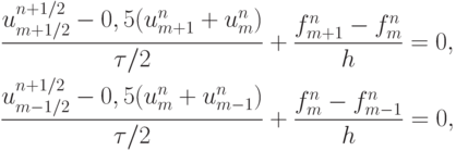
Generalization Lax-Wendroff schemes(predictor-corrector scheme). For quasi-linear equations (as well as linear equations with variable coefficients, inhomogeneous equations, etc.), the Lax-Wendroff scheme becomes more complex. To construct it, it is necessary to introduce the so-called half-integer points (points with fractional indices). At the first stage (predictor), the values ​​at half-integer points are calculated according to the above scheme - a generalization of the Lax scheme to the quasi-linear case:

at the second stage (corrector), the "leapfrog" scheme is used (a three-layer scheme on a cruciform template, which is not included in the family (3.8)):

The Lax-Wendroff scheme belongs to the so-called central schemes. Its pattern is symmetrical. At the first stage, the values ​​of the grid function are calculated at half-integer points of the template on the intermediate layer (t m - 1/2 , x m - 1/2) , (t n + 1/2 , x m + 1/2) , at the second stage the solution is calculated on the upper layer at the point (t n + 1 , x m) . The scheme is stable under the Courant condition.

The Lax-Wendroff schemes for linear inhomogeneous equations are constructed similarly.

McCormack's non-central scheme(predictor - corrector).

Like the Lax-Wendroff scheme above, the McCormack scheme has two stages. Consider the construction of the McCormack scheme for homogeneous equation(3.7). The first stage (predictor) has the form

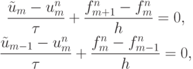
those. the scheme "explicit right corner" is used. The second stage is the corrector:

Thus, the calculation at the first stage according to the "right corner" scheme, at the second - "left corner".

Another McCormack scheme has the form

Such differential schemes are called non-central. Their advantages include the absence of half-integer indices, a simpler setting boundary conditions. In the linear case, the McCormack schemes coincide with the Lax–Wendroff scheme. The schemes have the second order of approximation in both variables, the schemes are stable under the Courant condition.

Rusanov's scheme(central scheme of the third order of accuracy).

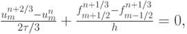
To construct the Rusanov scheme, not only half-integer points are introduced, but also two layers of intermediate points with fractional indices. The first stage of the Rusanov scheme (transition to layer 1/3) has the form

its second stage is the "leapfrog" scheme

and the third stage

At the first stage, the calculation is carried out according to the Lax scheme, at the second - according to the "cross" ("leapfrog") scheme. The last term of the third stage is introduced to ensure the stability of the scheme (a term proportional to the difference approximation of the 4th derivative).

The scheme is conditionally stable under the Courant condition and the condition .

non-central warming-cutler-lomax scheme 3rd order of accuracy.

First stage:

Second phase:

Third stage:

The last term is added for the stability of the circuit, which is conditionally stable under Courant's conditions.

Size: px

Start impression from page:

transcript

2 MINISTRY OF EDUCATION AND SCIENCE OF THE RUSSIAN FEDERATION NOVOSIBIRSK STATE UNIVERSITY Faculty of Mechanics and Mathematics Department of Mathematical Modeling G. S. Khakimzyanov, S. G. Cherny CALCULATION METHODS Part 4. Numerical methods for solving problems for equations of hyperbolic type Textbook Novosibirsk 014

3 LBC V.193 UDC X 16 Reviewer Ph.D. Phys.-Math. Sciences A. S. Lebedev vocational education"Novosibirsk State University» for years. X 16 Khakimzyanov, G. S. Computational methods: At 4 o'clock: textbook. allowance / G. S. Khakimzyanov, S. G. Cherny; Novosib. state un-t. Novosibirsk: RIC NGU, 014. Part 4: Numerical methods for solving problems for equations of hyperbolic type. 07 p. ISBN The textbook corresponds to the program of the course of lectures "Methods of Computation", which is read at the Faculty of Mechanics and Mathematics of Novosibirsk State University. In its fourth part, the fundamentals of numerical methods for solving initial-boundary value problems for equations of hyperbolic type are outlined, problems for seminars are formulated, samples of tests and tasks for practical exercises on a computer are given. The manual is intended for students and teachers of mathematical specialties of higher educational institutions. ISBN BBC V.193 UDC c Novosibirsk State University, 014 c G. S. Khakimzyanov, S. G. Cherny, 014

4 CONTENTS Preface Schemes for the linear transport equation Monotonicity property of difference schemes Construction of monotone schemes based on the differential approximation method Schemes for the nonlinear transport equation Schemes on an adaptive grid for the transport equation Difference schemes for the equation of string vibrations Difference schemes for a hyperbolic system of equations with constant coefficients Difference schemes for systems of nonlinear equations shallow water Difference schemes for problems of gas dynamics Test work on the topic "Investigation of difference schemes for the transport equation" Tasks for laboratory work Answers, instructions, solutions Bibliographic list

5 Preface In the fourth part of the manual, the fundamentals of numerical methods for solving initial-boundary value problems for equations of hyperbolic type are outlined, tasks on this topic for seminars are formulated, tasks for practical exercises on a computer and an example control work. Theoretical questions are stated rather briefly. For a deeper study of the issues under consideration, we recommend referring to the textbook by S. K. Godunov and V. S. Ryabenky, as well as to the books of G. I. Marchuk, A. A. Samarsky, A. A. Samarsky and A. V. Gulin , A. A. Samarsky and E. S. Nikolaev, B. L. Rozhdestvensky and N. N. Yanenko and textbooks published at NSU. The lectures deal with theoretical issues related to the study of only finite-difference schemes. As examples, schemes are considered for a linear transport equation, a first-order nonlinear scalar equation, a second-order equation describing string vibrations, a first-order linear system of equations, a system of nonlinear shallow water equations, and gas dynamics equations. Each paragraph is accompanied by tasks that need to be solved in the seminars. Many problems are provided with instructions and detailed solutions. Additional materials for seminars can be found in problem books. The manual provides examples of tasks for practical exercises in computer classes, gives recommendations on how to complete tasks, and discusses issues related to developing programs and presenting results. Additional tasks can be taken from teaching aids. The fourth part of the manual has an independent continuous numbering of paragraphs and figures and an independent bibliographic list. Inside paragraphs for formulas and statements (lemmas and theorems), two-index numbering is used, for example 4. 4.) from the manual "we write" according to the formula (1.4.)", instead of "by theorem 8.3 from the manual" "by theorem.8.3". The authors express their deep gratitude to the referee Alexander Stepanovich Lebedev for valuable advice and critical remarks, which contributed to the improvement of this paper. study guide. 4

6 1. Schemes for the linear transport equation 1.1. Some information from the theory of hyperbolic systems. Consider the Cauchy problem for a linear system of first-order differential equations u t + A u = f(x, t),< x <, 0 < t T, x u(x, 0) = u 0 (x), < x <. (1.1) Здесь u = (u 1,..., u m) T m-мерная вектор-функция переменных x, t, A вещественная m m матрица с элементами a i (x, t). Определение. Систему уравнений (1.1) будем называть гиперболической в некоторой области переменных (x, t), если в каждой точке этой области собственные значения λ 1, λ,..., λ m матрицы A вещественны и различны. Определение. Интегральная кривая x = x k (t) обыкновенного дифференциального уравнения dx dt = λ k(x, t) (1.) называется k-ой характеристикой системы уравнений (1.1). Предполагается, что элементы матрицы A обладают гладкостью, достаточной для того, чтобы через каждую точку плоскости (x, t) проходила единственная характеристика, отвечающая собственному значению λ k. Характеристики, проведенные через точку (x, t) (t >0) in the direction of decreasing time t, cross the Ox axis at m different points. Let us order the eigenvalues ​​of the hyperbolic system (1.1) (λ 1 (x, t)< λ (x, t) <... < λ m (x, t)) и через обозначим отрезок оси Ox, ограниченный точками пересечения этой оси с m-ой и первой характеристиками. Определение. Областью зависимости точки (x, t) для системы уравнений (1.1) называется множество точек верхней полуплоскости, ограниченное крайними характеристиками x = x m (t), x = x 1 (t) и отрезком . Область зависимости точки (x, t) изображена на рис. 1, а. Решение u системы (1.1) в точке (x, t) будет зависеть только от значений u 0 (x) на 5

7 segment. Therefore, if the initial data outside the interval is changed to others, then the solution at the point (x, t) will not change. Definition. The area of ​​influence of the point (x 0, 0) is the set of points (x, t) of the upper half-plane, bounded by the extreme characteristics of the system (1.1) emerging from (x 0, 0), i.e., the characteristics corresponding to the eigenvalues ​​λ 1 and λ m. The area of ​​influence of the point (x 0, 0) is shown in fig. 1b. If the initial data is changed only at the point (x 0, 0), then the solution of the hyperbolic system will change only at the points (x, t) belonging to the area of ​​influence of the point (x 0, 0). Let us now assume that instead of the Cauchy problem (1.1), we need to solve the initial-boundary value problem on the segment . Then, in addition to the initial conditions, it is necessary to set the boundary conditions. The number of boundary conditions on each of the boundaries is determined by the number of characteristics included inside the area. For example, if m 0 characteristics enter through the left boundary x = 0, i.e., m 0 eigenvalues ​​λ k are positive at x = 0, then m 0 boundary conditions must be specified on this boundary. If on the boundary x = l the number of negative eigenvalues ​​is equal to m l and, consequently, exactly m l characteristics enter the domain through the right boundary, then m l boundary conditions must be specified on this boundary. Since the eigenvalues ​​depend on time, the number of boundary conditions on each of the boundaries can change with time. t dx dt = m λ m (x,t) dx dt = λ 1 t dx dt =λ 1 dx dt = m λ x l a x r x (x 0.0) b x 1. Characteristics of the system of equations (1.1), limiting the areas of dependence of the point (x, t) (a) and the influence of the point (x 0, 0) (b) 6

8 Consider now the homogeneous hyperbolic system of equations (1.1) with constant coefficients. For a constant matrix A, its eigenvectors and eigenvalues ​​are constant, i.e., do not depend on x and t. Let l k be the k-th left eigenvector of matrix A corresponding to its eigenvalue λ k: l k A = λ k l k (k = 1,..., m). Multiply system (1.1) from the left by the vector l k: or where l k u t + l ka u x = 0. This equation can be written as follows: l k u t + λ k l k u x s ​​k t + λ s k k x = 0, = 0, (1.3) s k = l k u, k = 1,...m. (1.4) The solution s k (x, t) of equation (1.3) is transferred along the characteristic without change and therefore is calculated for t > 0 from the initial value s k at the point of intersection of the kth characteristic with the axis Ox: s k (x, t) = s k ( x λ k t, 0). (1.5) Functions s k are called Riemann invariants. 1. Linear shallow water model. The simplest mathematical model within which the motion of a fluid with surface waves can be described is the linear model of shallow water: η t + u 0 = 0, (1.6) x u t + g η = 0, (1.7) x η(x, 0) = η 0 (x), u(x, 0) = u 0 (x), (1.8) , η 0 (x) and u 0 (x) elevation and velocity at the initial time t = 0, 0 = const pool depth, g = const free fall acceleration. 7

9 The system of equations (1.6), (1.7) can be written as a homogeneous system (1.1) with matrix A and solution vector u: A = (0 0 g 0) (η, u = u). (1.9) The matrix A has two different real eigenvalues ​​λ 1 = c 0, λ = c 0 = g 0, (1.10) therefore the system of equations (1.6), (1.7) is of hyperbolic type. The characteristic equations (1.) take the following form: dx dt = c 0, dx dt = c 0, (1.11) therefore the characteristics are straight lines. The characteristics passing through the point (x, t), t > 0, intersect the Ox axis at the points x l and x r, where x l = x c 0 t, x r = x + c 0 t. (1.1) The left eigenvectors of the matrix A corresponding to the eigenvalues ​​(1.10) are given by the formulas l 1 = (c 0, 0), l = (c 0, 0). (1.13) y 0 η y= (x,t) l x y=- 0 initial dependent variables is given by the formulas r = c 0 η 0 u, s = c 0 η + 0 u, (1.14) 8

10 whence η = r + s c 0, u = s r 0. (1.15) From formula (1.5), taking into account equalities (1.14), we obtain formulas for solving the Cauchy problem in the invariants r(x, t) = r(x λ 1 t, 0) = r(x + c 0 t, 0) = c 0 η 0 (x r) 0 u 0 (x r), (1.16) s(x, t) = s(x λ t, 0) = s(x c 0 t, 0) = c 0 η 0 (x l) + 0 u 0 (x l). (1.17) Finally, using relations (1.15), we obtain the exact solution of the Cauchy problem (1.6), (1.7), (1.8) η(x, t) = η 0(x l) + η 0 (x r) + 0 u0( x l) u 0 (x r), c 0 u(x, t) = u 0(x l) + u 0 (x r) + c 0 η0(x l) η 0 (x r). 0 (1.18) When solving the initial-boundary value problem under consideration, it is necessary to set one condition at each end of the segment . Let us, for example, assume that the walls of the pool are impermeable to the liquid, which means that the velocity of the liquid on these walls is equal to zero: u(0, t) = u(l, t) = 0. (1.19) on the motion of a fluid with surface waves in a bounded basin: find a solution η(x, t), u(x, t) continuous in a closed region D = of the following initial-boundary value problem η t + u 0 x = 0, u t + g η = 0, 0< x < l, 0 < t T, x u(0, t) = u(l, t) = 0, 0 t T, η(x, 0) = η 0 (x), u(x, 0) = u 0 (x), 0 x l. (1.0) 1.3. Линейное уравнение переноса. Итак, если матрица A однородной гиперболической системы уравнений (1.1) постоянна, то такую систему можно свести к системе уравнений в инвариантах Римана, 9

11, the equations for the Riemann invariants do not depend on each other and each of them has the form u t + au x = 0, a = const. (1.1) This equation is the simplest hyperbolic equation and is called the linear transport equation. This equation can be used to study the properties of difference schemes used to solve hyperbolic systems of equations. Consider for the linear transport equation (1.1) the Cauchy problem u t + au x = 0,< x <, 0 < t T, u(x, 0) = u 0 (x), < x <. (1.) Характеристика x = x(t) уравнения (1.1) определяется уравнением dx dt = a, (1.3) т. е. является прямой с наклоном a к оси Ot. Следовательно, точное решение задачи Коши определяется по формуле u(x, t) = u 0 (x at). (1.4) График точного решения в момент времени t получается переносом графика начальной функции на величину at (в положительном направлении оси Ox, если a >0 and vice versa). For the transport equation with a constant coefficient a, it is easy to write out the exact solution for the initial-boundary value problem as well. Let, for example, a = const > 0. Then the following initial-boundary value problem u t + au x = 0, 0 is well-posed< x l, 0 < t T, u(0, t) = µ 0 (t), 0 t T, u(x, 0) = u 0 (x), 0 x l, u 0 (0) = µ 0 (0). (1.5) Легко проверить, что если u 0 (x) и µ 0 (t) дифференцируемые функции, то решение задачи (1.5) определяется формулой u(x, t) = { u0 (x at) при t x/a, µ 0 (t x/a) при t x/a. (1.6) 1.4. Явная противопоточная схема. Перейдем теперь к изучению конечно-разностных схем решения линейного уравнения переноса. 10

12 Let's start with an explicit scheme with upstream differences (upstream scheme) for the initial-boundary value problem u t + au x = f(x, t), 0< x l, 0 < t T, a = const >0, u(0, t) = µ 0 (t), 0 t T, u(x, 0) = u 0 (x), 0 x l, u 0 (0) = µ 0 (0). (1.7) In what follows, we will consider only uniform grids covering the closed domain D = . Let us construct the following difference scheme u n + a un un 1 = f n, = 1,..., N, u n 0 = µ n 0, n = 0,..., M, u 0 = u 0(x), = 0 ,..., N, (1.8) approximating problem (1.7) with order O(+). As before, this scheme can be written in operator form L u = f. The name of the upwind scheme is due to the fact that if we consider the transport equation as a model equation for a system of equations describing the flow of a liquid or gas, and identify the coefficient a with the fluid velocity, then at a positive velocity, i.e., at a > 0, in the scheme left difference derivatives are taken using the node x 1 located upstream of the "stream" (located upstream). Let us introduce uniform norms in the space of grid functions U and the space of right-hand sides F: where f F (= max u U max n u n C = max 0 N un, = max n un C, (1.9)) µn 0, ​​(u 0) C, max f n n C, (1.30) f n C = max 1 N f n uniform norms on the layer t = t n. Using the maximum principle, we can prove the following assertion. Theorem 1.1. Satisfaction of condition a 1 (1.31) 11

13 is sufficient for the stability of the upwind scheme (1.8) in the uniform norm. Proof. Let x be a grid node with number 1 N. Let us rewrite the difference equation of the circuit at this node = (1 r)u n + ru n 1 + f n, where r = a/. It follows from the conditions of the theorem that 1 r 0, so the following estimate (1 r) u n +r u n 1 + f n (1 r) u n C +r u n C + f n C u n C + max m f m C will be valid. At the boundary node, we have the following estimate 0 = µ n+1 0 max m µm 0. Therefore, the maximum of the left-hand sides of these inequalities cannot exceed the maximum of the two numbers on the right-hand sides of these inequalities: (C max max m) µm 0, u n C + max f m m C, and this is the maximum principle. We have found that, under condition (1.31), scheme (1.8) satisfies the maximum principle. Therefore (see Theorem 3.1.1) it will be stable in the uniform norm in the initial data, boundary conditions, and on the right-hand side. The same condition (1.31) is also a necessary condition for the stability of scheme (1.8), which follows from the Neumann spectral criterion for stability. Let's prove it. Let us take the harmonic u n = λ n e iφ (1.3) and substitute it into the homogeneous difference equation. As a result, for the transition factor we obtain the equation Therefore, λ = 1 r (1 e iφ) = 1 r(1 cos φ) ir sin φ. λ = 1 r(1 cos φ) + r (1 cos φ) + r sin φ = 1

14 = 1 r(1 cos φ) [ r(1 cos φ) r(1 + cos φ)] = 1 r(1 cos φ)(1 r). Let the steps and in scheme (1.8) be related by the passage to the limit r = a = const. (1.33) Then the eigenvalues ​​λ (φ) do not depend on, so the necessary Neumann stability condition reduces to the requirement or λ (φ) 1, φ R. (1.34) r(1 cos φ)(1 r) 0, φ R. (1.35) Obviously, this inequality is equivalent for a > 0 to condition (1.31). Thus, condition (1.31) for a > 0 is a necessary and sufficient condition for the stability of the upwind scheme in the uniform norm. Note that for a< 0 схема (1.8) абсолютно неустойчива, поскольку в этом случае нарушается неравенство (1.34) (см. задачу 1.1). Какую же схему следует использовать при a < 0, когда поток распространяется справа налево? Отметим, что в этом случае корректной будет такая начально-краевая задача u t + au x = f(x, t), 0 x < l, 0 < t T, a = const < 0, u(l, t) = µ l (t), 0 t T, u(x, 0) = u 0 (x), 0 x l, u 0 (l) = µ l (l). (1.36) Для этой задачи возьмем следующую противопоточную схему u n + a un +1 un = f n, = 0,..., N 1, u n N = µn l, n = 0,..., M, u 0 = u 0(x), = 0,..., N, (1.37) которая аппроксимирует дифференциальную задачу (1.36) с порядком O(+). Используя принцип максимума и спектральный признак Неймана, можно показать, что схема (1.37) при a < 0 будет устойчива при выполнении условия a 1. С другой стороны, при a >0 scheme (1.37) will be absolutely unstable (see problem 1.). 13

15 Thus, we have constructed two conditionally stable explicit schemes with upstream differences for the transport equation with a constant coefficient a u n u n + a un un 1 + a un +1 un. They are stable under the inequality = f n, if a > 0, = f n, if a< 0. (1.38) a 1. (1.39) Во внутренних узлах сетки противопоточную схему (1.38) можно записать в виде одного уравнения u n + a + a u n un 1 + a a u n +1 un = f n. (1.40) Аналогично выглядит явная противопоточная схема и в случае знакопеременного коэффициента a(x, t). Например, если на границах отрезка выполнены условия a(0, t) >0, a(l, t)< 0, 0 t T, то получим такую противопоточную схему где u n + a + un un 1 + a un +1 un = f n, = 1,..., N 1, u n 0 = µ n 0, u n N = µ n l, n = 0,..., M, (1.41) u 0 = u 0 (x), = 0,..., N, a + = an + a n, a = an a n, (1.4) которая аппроксимирует с порядком O(+) начально-краевую задачу u t + a(x, t)u x = f(x, t), 0 < x < l, 0 < t T, u(0, t) = µ 0 (t), u(l, t) = µ l (t), 0 t T, u(x, 0) = u 0 (x), 0 x l. (1.43) 14

16 With the help of the maximum principle, one can prove (see problem 1.10) that for the stability of the upwind scheme (1.41) with a variable coefficient a(x, t) it is sufficient to satisfy the condition max a(x, t) 1. (1.44) x,t 1.5 . Lax's scheme. Further, for simplicity of presentation, we will consider the initial-boundary value problem (1.7) with the homogeneous transport equation u t + au x = 0. (1.45) In the Lax scheme, the difference equation approximating the transport equation (1.45) is written as 0.5 (u n +1 + ) un 1 + a un +1 un 1 = 0, = 1,..., N 1. (1.46) For the local approximation error, we have the expression ψ n, = u tt u xx +..., therefore, for = O( ) the Lax scheme will not approximate the transport equation, but under the law of passage to the limit r = a = const (1.47) it will approximate with the order O(+). Thus, approximation takes place only for a certain connection between the steps and, i.e., the Lax scheme belongs to the class of conditionally approximating schemes. For the transition factor, we obtain the formula λ(φ) = cos φ ir sin φ. Therefore, under the law of passage to the limit (1.47), the necessary condition for the stability of the Lax scheme is the fulfillment of the inequality r 1, i.e., a 1. (1.48) 15

17 1.6. Diagram of Lax Wendroff. The difference equations of this scheme look like this: u +1/ 0.5 (u n +1 +) un + a un +1 un = 0, / u n + a u +1/ (1.49) u 1/ = 0. Lax Wendroff’s scheme refers to family of two-step schemes. In this scheme, first, at half-integer nodes x +1/ = x +/, auxiliary quantities u +1/ related to the time t n + / are calculated according to the Lax scheme. Then, at the second step, the values ​​of the desired grid function are calculated at the (n + 1)th time layer. To study the approximation and stability of two-step schemes, the auxiliary quantities u are preliminarily excluded from the scheme. As a result of the elimination, we obtain the one-step scheme of Lax Wendroff u n + a un +1 un 1 = a un +1 un + un 1, (1.50) which, as it is easy to check, approximates the transport equation (1.45) with the second order in u. For the transition factor, we have the following expression λ = 1 ir sin φ r sin φ. Therefore, the necessary stability condition λ 1 will be equivalent to the fulfillment of the inequality (1 r sin φ) + r sin φ 1, or 1 4r sin φ + 4r4 sin 4 φ + 4r sin φ (1 sin φ) 1. The latter inequality is equivalent to the condition r 1. Thus, the necessary condition for the stability of the Lax Wendroff scheme coincides with the necessary condition (1.48) for the stability of the Lax scheme Dissipation and dispersion. Along with the transport equation u t + au x = 0, a = const (1.51) 16

18 consider two more equations u t + au x = µu xx, µ = const > 0, (1.5) u t + au x + νu xxx = 0, ν = const. (1.53) Let the initial function in the Cauchy problem for these equations be represented as a Fourier series u(x, 0) = m b m e imx. (1.54) We will seek the solution of each of these equations by the method of separation of variables u(x, t) = b m λ t e imx = b m u m (x, t), (1.55) m m where u m (x, t) is a harmonic with wavenumber m u m (x , t) = λ t e imx, (1.56) λ is to be determined. The real and imaginary parts of the harmonic are m-waves, the length l of which is related to the wave number by the formula l = π m. (1.57) Since equations (1.51) (1.53) are linear, the behavior of each of the harmonics can be considered independently. Substituting the harmonic with wavenumber m into the transport equation (1.51), we obtain either ln(λ) + aim = 0 λ = e aim. Therefore, if the harmonic (1.56) is a solution of the transport equation, then it has the form Denoting ξ = x at, we obtain um (x, t) = e im(x at). (1.58) u m (x, t) = e imξ = um (ξ, 0). (1.59) 17

19 Thus, at any time t > 0, the harmonic u m is obtained by shifting the initial harmonic by at. Therefore, the transport equation describes the motion of m-waves, which, regardless of their length, propagate at a constant speed v m = a without distorting their shape. It is easy to check that the harmonic (1.56) is a solution to the second equation (1.5) if ln(λ) + aim = µm or λ = e aim e µm, i.e., the harmonic in this case has the form u m (x, t) = e µmt e im(xat). Consequently, for all harmonics, the wave amplitude decays (wave dissipation). Since m = π/l, short waves decay faster than long ones. Velocity v m of wave propagation does not depend on the wavelength and is still equal to a. The term µu xx with the second derivative of the solution is responsible for the wave dissipation. Finally, substituting the harmonic into equation (1.53) gives ln(λ) + aim + ν(im) 3 = 0, or whence we obtain that λ = e im(a νm), u m (x, t) = e im(x ( a νm)t). Thus, the third equation describes the wave motion without changing its amplitude (without dissipation). But the speed of its propagation depends on the wavelength v m = a νm. (1.60) This formula shows that waves of different lengths propagate with different speeds (waves disperse). The velocity of propagation of short-wave disturbances (large m) undergoes more significant changes. The term νu xxx with the third derivative of the solution is responsible for the wave dispersion. 18

20 Having considered the behavior of individual harmonics, we can now predict the qualitative behavior of the solution (1.55) of the Cauchy problem for these equations. Let, for example, the initial function u(x, 0) have the form of a step ( 1, x 0, u(x, 0) = (1.61) 0, x > 0 and a > 0. The expansion of such a function in the Fourier series (1.54) will contain the entire set of harmonics.The solution of the Cauchy problem for the transport equation (1.51) is represented in the form the solution of the problem is the initial profile moving with velocity a. Solution u(x, t) = m b m e µmt e im(x at) = m b m e µmt e imξ (1.63) of the Cauchy problem for equation (1.5) with a dissipative term in which short waves strongly u(x, t) = m b m e im(x (a νm)t) (1.64) of the Cauchy problem for equation (1.53), in which waves of different lengths move with different speeds, has a nonmonotonic, oscillating character. According to formula (1.60), for ν > 0, waves of small length will have a velocity lower than waves of large length, and for ν< 0 наоборот. Поэтому осцилляции будут отставать от основного решения (описываемого первыми гармониками) при ν >0 and, accordingly, move ahead as ν< Дифференциальное приближение разностной схемы. Вернемся к численному решению задачи Коши для уравнения переноса (1.51). В качестве начального профиля возьмем ступеньку { 1, x x0, u(x, 0) = (1.65) 0, x >x 0 19

21 and carry out the calculation according to the explicit upwind scheme u n + a un un 1 = 0, a = const > 0. (1.66) As a result, we obtain a solution in the form of a smeared step (Fig. 3), i.e., the solution will be qualitatively the same as and the solution of equation (1.5) with a dissipative term. What's the matter? After all, we wanted to solve the transport equation, in which there is no dissipative term. The point is that we were looking numerically for a solution not to the transport equation, but to a solution to a difference scheme. Thus, the properties of the solutions of the differential equation being approximated and the approximating difference equation may not coincide. How, then, to predict the properties of the solution of the difference equation? y x 30 Fig. Fig. 3. Graphs of the exact solution (dashed lines) and numerical solution (solid lines) obtained using the upwind scheme (1.66) at time points t = 1 (1); t=8(); t = 15 (3). a = 1; x0 = 10; a/ = 0.5 This can be done using the differential approximation method, which we will now briefly review. The essence of this method is to replace the original difference equation with a special differential equation that has all the properties of the difference equation under study. Therefore, instead of studying the difference equation, this differential equation is investigated, which in many cases is much easier to do. Obtaining a differential equation corresponding to a difference equation begins with writing this difference equation in the form of a so-called theoretical difference scheme, in which difference operators act in the same functional space as the differential operators they approximate. For example, the difference equation (1.66) is written as the following theoretical difference 0

22 schemes u(x, t +) u(x, t) u(x, t) u(x, t) + a = 0. (1.67) The solution of such a scheme is the function u(x, t) of continuous arguments x and t while the solution of equation (1.66) is the grid function u, defined only at the grid nodes. Let a sufficiently smooth function u(x, t) be a solution of the theoretical difference scheme (1.67). We substitute it into this scheme and express u(x, t +) and u(x, t) in terms of the values ​​of the function and its derivatives at the point (x, t) using the Taylor formula. As a result, we obtain a differential equation equivalent to the difference scheme (1.67) u t + au x + u tt + 6 u ttt a u xx + a 6 u xxx +... = 0. (1.68) Definition. The differential equation of infinite order (1.68) obtained after expanding the solution u(x, t) of the theoretical difference scheme (1.67) by the Taylor formula is called the differential representation of the difference scheme (1.66). Some properties of the difference scheme can already be studied with the help of this differential representation, but for our purposes it will be more convenient to use another form of the differential representation, which results from the elimination of all time derivatives from (1.68) except for the one that enters the approximated equation (1.51), m i.e. except for u t. Let us show, for example, how to eliminate the time derivatives in terms of order u. To do this, we rewrite equation (1.68) taking into account the terms up to the order O() and O() u t + au x + u tt + 6 u ttt a u xx + a 6 u xxx = O() (1.69) and use the resulting equation to find derivative u t: u t = au x u tt 6 u ttt + a u xx a 6 u xxx + O() (1.70) We substitute this derivative into the terms of equation (1.69) containing the derivatives (u t) t and (u t) tt. Taking into account the order of smallness of the coefficients at the second and third derivatives with respect to time, we obtain that in (u t) t 1

23 it suffices to substitute the derivative (1.70) calculated with O(+) accuracy: u t = au x u tt + a u xx + O(+), (1.71) and in (u t) tt with O(+) accuracy: u t = au x +O(+). (1.7) As a result of such a substitution, equation (1.69) takes the following form: u t + au x + (au x u tt + a) u xx + t 6 (au x) tt = = a u xx a 6 u xxx + O(), or u t + au x a u tx 4 u ttt + a 4 u txx a 6 u ttx = = a u xx a 6 u xxx + O(). (1.73) After substituting into equation (1.69), we then take similar actions with equation (1.73). Now we need to substitute the derivative u t, determined from equation (1.73), into the four terms of the same equation: u t + au x a (au x + a u tx + a u xx) x 4 (au x) tt + + a 4 (au x) xx a 6 (au x) tx = a u xx a 6 u xxx + O(). After reducing similar ones, we obtain the equation u t + au x a 1 u txx + a 4 u ttx = = a (a) (1 r) u xx + a u xxx + O(), 6 (1.74) in which, in contrast to (1.69) , there are no second time derivatives. The mixed derivatives u txx and u ttx remaining in (1.74) can be calculated on the basis of equality (1.7): u txx = au xxx + O(+), u ttx = a u xxx + O(+). (1.75)

24 Therefore, the differential representation (1.74) takes the form u t + au x = a (1 r)u xx a 6 (r 3r + 1)u xxx + O(). (1.76) Thus, we got rid of time derivatives with powers of and. But the derivatives with respect to t have so far remained at higher powers on the right side of O(). If we continue the described procedure further, then in the representation (1.68) we can remove time derivatives up to an arbitrarily high order. As a result, we obtain a differential representation of the circuit in the form or u t + au x = a (1 r)u xx + a 6 (1 r)(r 1)u xxx +... (1.77) u t + au x = k= c k k u x k . (1.78) Definition. The equation of infinite order (1.78) is called the P-form of the differential representation of the difference scheme. Let the difference scheme have orders of approximation γ 1 and γ in and respectively. Definition. The differential equation obtained from the P-form of the differential representation by discarding terms of order O(γ1+1, γ+1) and higher is called the first differential approximation (p.d.p.) of the difference scheme. For the upwind scheme (1.66), the p.d.p. is a second-order differential equation u t + au x = µu xx, µ = a (1 r), (1.79) which, as we see, coincides with equation (1.5) with a dissipative term . Thus, for r 1, our scheme implicitly introduces viscosity (dissipation) into the approximated transport equation, which is called the approximate or scheme viscosity. The presence of approximation viscosity leads to smearing of the initial step. Definition. The property of a difference scheme due to the presence of even-order derivatives in its pdp is called numerical dissipation. 3

25 The P-form of the differential representation of the Lax Wendroff difference scheme has the form + νu xxx = 0, ν = a 6 (1 r) (1.80) coincides with equation (1.53) with a dispersion term. Consequently, at r 1, the Lax Wendroff scheme implicitly introduces dispersion into the approximate transport equation, so the solution of the difference scheme can oscillate (Fig. 4). y Fig. Fig. 4. Graphs of the exact solution (dashed lines) and numerical solution (solid lines) obtained using the Lax Wendroff scheme at time points t = 1 (1); t=8(); t = 15 (3). a = 1; x0 = 10; a/ = 0.5 Definition. The property of a difference scheme, due to the presence of odd-order derivatives in its pdp, is called numerical dispersion. Let's summarize our reasoning. For problems with a smoothly varying solution, in which the contribution of high-frequency harmonics is small, the accuracy of the Lax Wendroff scheme is higher than that of the upwind scheme. If we solve numerically a problem in which the solution has a sharply changing monotonic profile, then applying the first-order upwind scheme will give a monotonic non-oscillating profile, but strongly smoothed. This is the result of numerical dissipation. Lax Wendroff's scheme, which has numerical dispersion, can give nonmonotonic profiles of the numerical solution in the vicinity of a discontinuity or a sharp change in the solution, distorted by nonphysical oscillations. x4

26 CHALLENGES 1.1. Show that for a< 0 схема (1.8) абсолютно неустойчива. 1.. С помощью спектрального метода Неймана показать, что явная схема для уравнения (1.1) u n + a un +1 un = 0, n = 0,..., M 1, = 0, ±1, ±,... (1.81) при a >0 is absolutely unstable Using the Neumann spectral method, derive the necessary condition for the stability of the three-layer “leap-frog” scheme (scheme with stepping over, “leap frog” scheme) for equation (1.1) u n 1 + a un +1 un 1 = 0, n = 1, ..., M 1, = 0, ±1, ±,..., (1.8) if the law of passage to the limit is given in the form (1.33) Determine the order of approximation of the explicit scheme with central difference u n + a un +1 un 1 = 0 , (1.83) constructed for the transport equation (1.1). Using the Neumann spectral method, investigate the stability of this scheme if the law of passage to the limit is given in the form a = const. (1.84) 1.5. Determine the order of approximation of the majorant scheme u n + a un +1 un 1 = a un +1 un + un 1, (1.85) constructed for the transport equation (1.1). Using the Neumann spectral method, investigate the stability of this scheme if the passage to the limit law is given in the form (1.84). 5

27 1.6. Determine the order of approximation of the McCormack scheme u un + a un +1 un = 0, 0, 5 (u +) un / + a u u 1 = 0, (1.86) constructed for the transport equation (1.1). Using the Neumann spectral method, investigate the stability of this scheme if the passage to the limit law is given in the form (1.84) Determine the order of approximation of the upwind scheme with weights u n + σa un (1 σ)a un un 1 = 0, (1.87) constructed for the transport equation ( 1.1) with coefficient a > 0. Using the Neumann spectral method, derive a necessary condition for the stability of scheme (1.87) if the passage to the limit law is given in the form (1.84) Using the maximum principle, investigate the stability in the uniform norm of the implicit upwind scheme u n + a un+1 1 = f n+1, = 1,..., N, u n 0 = µ n 0, n = 0,..., M, u 0 = u 0(x), = 0,..., N , (1.88) constructed for problem (1.7) Using the maximum principle, find a sufficient condition for stability in the uniform norm of an upwind scheme with weights u n + σa un (1 σ)a un un 1 = f n+1/, u n 0 = µ n 0 , n = 0,..., M, u 0 = u 0(x), = 0,..., N, (1.89) constructed for problem (1.7). Here 0 σ 1. 6

28 1.10. Using the maximum principle, prove that the fulfillment of condition (1.44) is sufficient for the stability of the upwind scheme (1.41) with a variable coefficient a(x, t) scheme u n + a un+1 1 = 0, (1.90) constructed for the transport equation (1.1) with coefficient a > 0. Give a qualitative explanation of the behavior of the difference scheme solution for t > 0 if at the initial time t = 0 a step ( 1.61).. Monotonicity property of difference schemes.1. One of the main requirements for difference schemes is that the solution of the difference equation must convey the features of the behavior of the solution of the differential equation being approximated. Consider, for example, the Cauchy problem for the linear transport equation u t + au x = 0, a = const > 0,< x <, t >0, (.1) u(x, 0) = u 0 (x). (.) If u 0 (x) is a nondecreasing (nonincreasing) function of the variable x, then for any fixed t > 0 the solution u(x, t) of problem (.1), (.) will also be a nondecreasing (nonincreasing) function of the variable x. This follows from the fact that at any time the solution is given by the formula u(x, t) = u 0 (x at). (.3) It is natural to require that the solution of the difference scheme approximating problem (.1), (.) also has a similar property. But it turns out that many difference schemes violate the monotonicity of the numerical solution: instead of the expected monotonic profiles, solutions containing nonphysical oscillations are obtained (Fig. 4). The reason for their occurrence is the numerical dispersion of the difference 7

29 schemes discussed in the previous paragraph. In this section, we present conditions under which the difference scheme will preserve the monotonicity of the numerical solution. Let us consider an arbitrary explicit difference scheme = α b α u n + α, (.4) where α is an integer, α = α 1, α 1 + 1,..., α, nodes x + α determine the template of the scheme. Definition. Difference scheme (.4) is called a scheme that preserves the monotonicity of the numerical solution (monotone scheme) if it transforms any monotone function u n into a monotone function on the (n + 1)th time layer, moreover, with the same direction of growth. Example 1. We approximate equation (.1) on a uniform grid by the upwind scheme u n + a un un 1 = 0. (.5) This scheme has the first order of approximation in u. Let the grid function u n on the nth time layer be monotone, for example, a monotonically increasing function, i.e., u n un 1 for an arbitrary. In this case, under the condition of stability of the circuit having the form aæ 1, where æ = /, we obtain + aæ(u n 1 u n) 0. Thus, the solution also increases monotonically on the (n + 1)th layer. Thus, the upwind scheme (having dissipation at aæ< 1) является схемой, сохраняющей монотонность. Пример.. Покажем, что схема Лакса Вендроффа (1.49) (не обладающая диссипацией при aæ < 1) не сохраняет монотонность численного решения. Пусть начальная функция для уравнения (.1) имеет вид (1.61) { 1, при x 0, u 0 (x) = 0, при x > 0. 8

30 Consequently, the initial grid function ( u 0 1, for 0, = u 0 (x) = 0, for > 0 is monotonically decreasing. Let us rewrite the considered scheme in the form of a one-step scheme (1.50), and then in the form of scheme (.4) with coefficients b 1 = a æ + aæ, b 0 = 1 a æ, b 1 = a æ aæ (.6) Then it is easy to see that equality 1 holds at the first time layer, for 1, u 1 b = 1 + b 0, at = 0, b 1, at = 1, 0, at. At aæ< 1 схема устойчива, но b 1 + b 0 >1, i.e., the grid function u 1 is not monotonically decreasing. The monotonicity of schemes for equations with constant coefficients can be investigated using the following theorem. Theorem.1. In order for the difference scheme (.4) with constant coefficients b α to remain monotonic, it is necessary and sufficient that the conditions b α 0 hold for all α. (.7) Proof. Necessity. Assume that scheme (.4) remains monotonic, but there exists a negative coefficient b α0< 0. Возьмем монотонно возрастающую функцию u n = { 0, < α0, 1, α 0. (.8) Тогда u0 n+1 1 = b α u n α b α u n 1+α = α α = b α b α = b α0 < 0, α α 0 α α

31 i.e., the function is not monotonically increasing, and, consequently, scheme (.4) does not preserve monotonicity, which contradicts the original assumption. The obtained contradiction proves that all coefficients b α are non-negative. Adequacy. Let b α 0 and u n be a monotone function, for example, a monotonically increasing function. Then 1 = α b α u n + α α b α u n 1+α = α b α (u n + α u n 1+α) 0, i.e., also a monotonically increasing function. Thus, scheme (.4) remains monotonic. Let us return again to examples 1 and ., and now we will not assume that a > 0. The upwind scheme for equation (.1) with an arbitrary sign of the coefficient a looks like this: where u n Rewrite it in the form (.4) + a + un un 1 a + = a + a + a un +1 un, a = a a. = 0, (.9) where = b 1 u n 1 + b 0 u n + b 1 u n +1, (.10) b 1 = æa +, b 0 = 1 æ a, b 1 = æa. If the stability condition a æ 1 (.11) is satisfied, all these coefficients are non-negative. In addition, they are constant, therefore, according to Theorem 1, the upwind scheme (.9) preserves the monotonicity of the solution under condition (.11). The Lax Wendroff scheme is stable under the same condition (.11) as the upwind scheme, and it can be written in the form (.10) with coefficients (.6), whence it is clear that under the condition a æ< 1 один из 30

32 coefficients b 1 or b 1 is negative. According to Theorem 1, this implies that the Lax Wendroff scheme, which has a second-order approximation with respect to u, does not preserve the monotonicity of the numerical solution. But perhaps there are other schemes of the second order of approximation, which have the property of monotonicity. It turns out that there are no such schemes. The paper shows that for the linear transport equation (.1) it is impossible to construct a monotone scheme with constant coefficients of the second order of approximation... Let us now consider scheme (.4) with variable coefficients b α. Will the condition (.7) of non-negativity of the coefficients be sufficient for such schemes to preserve the monotonicity of the numerical solution? It turns out not. Let's give a corresponding example. Example 3. Let the Cauchy problem be solved for the equation u t + a(x)u x = 0, (.1) where a(x) is a strictly increasing positive bounded function: 0< a(x) < 1 и a >0. To solve this problem, let us take a scheme with variable coefficients 0, 5 (u n +1 +) un 1 + a u n +1 un 1 = 0, (.13) where a = a(x), x is a node of the uniform grid. The above scheme is analogous to the Lax scheme (1.46), which preserves the monotonicity of the numerical solution (see Problem 1). We will assume that the condition æa< 1, (.14) гарантирующее устойчивость схемы (.13) в равномерной норме по начальным данным: C u 0 C. (.15) Запишем схему (.13) в виде (.4): = b 1, u n 1 + b 1, u n +1, (.16) где b 1, = 1 + æa, b 1, = 1 æa, 31

33, the coefficients b α are provided with an additional index, since they are variable coefficients and change when moving from one node to another. Due to condition (.14), both coefficients are positive, but scheme (.13) does not preserve the monotonicity of the numerical solution. Indeed, taking a monotonically increasing function ( u n 0,< 0, = 1, 0, убеждаемся, что на (n + 1)-м слое по времени имеет место равенство = 0, при < 1, b 1, 1, при = 1, b 1,0, при = 0, 1, при 1. Но b 1, 1 >b 1.0, so the grid function is increasing. is not monotone The above example shows that for schemes with variable coefficients other monotonicity criteria should be used than the criterion (.7) specified in Theorem.1. Theorem.. Let the coefficients of the difference scheme = b 1, u n 1 + b 0, u n + b 1, u n +1 (.17) satisfy the condition at each node x Then the fulfillment for all conditions b 1, + b 0, + b 1 , = 1. (.18) b ±1, 0, b 1, + b 1, 1 1 (.19) is necessary and sufficient for scheme (.17) with variable coefficients to preserve the monotonicity of the numerical solution. Proof. We write scheme (.17) with variable coefficients satisfying condition (.18) in the following form: = u n b 1, (u n u n 1) + b1, (u n +1 u n). (.0) 3

34 Then +1 = un +1 b 1,+1 (u n +1 u n) + b1,+1 (u n + u n +1). Therefore, +1 un+1 = (u n +1 u n) (1 b 1,+1 b 1,) + (+ b 1,+1 u n + u n (+1) + b 1, u n u n) (.1) 1. Necessity. Let scheme (.17) be monotone. Let us prove that its coefficients satisfy inequalities (.19). Suppose that this is not true and some of the conditions (.19) are not satisfied at some node x 0, for example b 1,0< 0. Положим Из (.1) тогда следует u n = { 0, если < 0, 1, если un+1 0 = b 1,0 < 0, т. е. функция не является монотонно возрастающей, что противоречит исходному предположению о монотонности схемы (.17). Аналогично проверяются и остальные неравенства в (.19). Достаточность. Пусть в каждом узле x коэффициенты схемы (.17) удовлетворяют неравенствам (.19) и функция u n является монотонной, например монотонно возрастающей. Тогда из равенства (.1) следует, что функция также будет монотонно возрастающей функцией. Теорема доказана. Нетрудно проверить, что коэффициенты схемы (.16) не удовлетворяют второму из условий (.19) теоремы.3, поэтому эта схема не является схемой, сохраняющей монотонность численного решения. Дадим другую формулировку теоремы.. Теорема.3. Для того чтобы конечно-разностная схема u n + C 1/ un x, 1/ C+ +1/ un x,+1/ = 0, (.) сохраняла монотонность численного решения, необходимо и достаточно выполнение при всех условий где æ = /, u n x,+1/ = un +1 un C ± +1/ 0, C +1/ + C+ +1/ 1 æ, (.3). 33

35 Proof. The scheme (.) can be rewritten in the form (.17), where b 1, = æc 1/, b 1, = æc + +1/, b 0, = 1 æc 1/ æc+ +1/. Then equality (.18) holds for the coefficients b α , and conditions (.19) are equivalent to conditions (.3). Comment. We prove that the fulfillment of inequalities (.3) is sufficient for the scheme (.) to be a TVD (Total Variation Diminising Sceme), i.e., a scheme whose solution u n for any n 0 satisfies the nonincreasing condition for the total variation TV () TV (u n), (.4) where the total variation of the grid function u n is understood as TV (u n) = u n +1 u n. (.5) At present, TVD schemes and their various modifications are used to solve many problems with discontinuous solutions. The reason for such a great popularity of these methods is that they give non-oscillating solution profiles, high resolution in the region of discontinuities, and retain high accuracy in regions of smoothness of the solution. Modern high-order TVD schemes are based on certain methods of restoring (reconstructing) the values ​​of functions at cell boundaries from their values ​​at the centers of neighboring cells. In this case, the circuit template is variable and depends on the behavior of the numerical solution. Reconstruction algorithms are based on the use of special flow limiters , which are built in such a way that the circuit with limiters has the TVD property (.4)..3. Monotonization of Lax Wendroff's scheme. If the initial function at t = 0 is given in the form of a step, then on the next time layers we will obtain, according to the Lax Wendroff scheme, a step distorted by oscillations (see Fig. 4). But it turns out that Lax Wendroff's scheme can be modified so that it has 34

36 TVD-property (.4), and hence, according to Theorem 3, would become a scheme that preserves the monotonicity of the numerical solution. However, the coefficients of the modified scheme will no longer be constant, they may depend on the solution on nth layer, i.e. the modified circuit will be non-linear. Consider the transport equation (.1) in the case a = const > 0. Lax Wendroff's scheme (1.50) can be rewritten as follows: u n +a un x,+1/ + un x, 1/ a () u n x,+1/ un x, 1/ = 0, (.6) or u n + au n x, 1/ + a (1 aæ) un x,+1/ un x, 1/ u n = 0, (.7) + au n x, = a (1 aæ) un xx,. (.8) P.d.p. (1.79) of the upwind scheme contains the dissipative term 0, 5a (1 aæ) u xx on the right-hand side, and in representation (.8) the same dissipative term in the difference form has the opposite sign. Thus, the Lax Wendroff scheme is represented as a monotonic scheme with an upstream difference, supplemented by the so-called anti-diffusion term, which eliminates the dissipative term in the PDP of the upwind scheme, turning it into the Lax Wendroff scheme. By decreasing the antidiffusion term at the places where oscillations may appear, one can try to prevent them. We regulate the antidiffusion term in the Lax Wendroff scheme (.7) using the limiter function Φ(ξ) of some argument ξ: u n +au n x, 1/ + a (1 aæ) ((Φu n x) +1/ (Φu n x) 1/) = 0. (.9) If Φ 0, then we have a monotone upwind scheme of the first order of approximation. If Φ 1, then we obtain the Lax Wendroff scheme of the second order of approximation on smooth solutions, but oscillating on discontinuous solutions. 35

37 In difference scheme (.9) Φ +1/ = Φ(ξ +1/). As a discrete argument ξ +1/ we choose the value u n x, 1/ ξ +1/ = u n for u n x,+1/ 0, x,+1/ (.30) 1 for u n x,+1/ = 0. On the oscillating solution the ratio u n x, 1/ /un x,+1/ becomes negative; therefore, for ξ +1/< 0 полагаем, что Φ +1/ = 0. Далее будем считать, что функция Φ = Φ(ξ) непрерывного аргумента ξ также принимает нулевые значения при ξ < 0. Более того, предполагая, что функция-ограничитель является непрерывной, полагаем, что Φ(ξ) 0 при всех ξ 0. Далее рассмотрим случай, когда ξ +1/ >0. We choose the limiter function in such a way that the scheme satisfies the TVD condition (.3) and preserves the second order of approximation on smooth solutions. To do this, we transform the modified Lax Wendroff scheme (.9) to the form (.): or u n + au n x, 1/ + a (1 aæ) ((Φ ξ u n [ + a aæ ((Φ) ξ) +1/ + 1/ Φ 1/) u n x, 1/ = 0, Φ 1/)] u n x, 1/ = 0. Thus, the coefficients of scheme (.9) written as (.) are determined by the formulas [ C + +1 / = 0, C 1/ = a aæ ((Φ))] ξ Φ 1/. +1/ According to Theorem 3, the condition 0 C 1/ 1 æ (.31) will guarantee that the Lax Wendroff scheme with the limiter function introduced into it will preserve the monotonicity of the numerical solution. Further, we assume that the stability condition for the Lak-36 scheme

Wendroff’s condition is satisfied, i.e., aæ 1. Then, in order for inequalities (.31) to be valid for all aæ 1, it is necessary and sufficient that the inequalities (Φ) ξ +1/ Φ 1/ hold, and for this it suffices to require that for all the following inequalities: (Φ) 0, 0 Φ +1/. ξ +1/ The region in the plane of variables Φ and ξ, in which these inequalities hold, is shown in Fig. 5, a. If the graph of the function Φ = Φ(ξ) lies in this region, then the modified scheme (.9) will preserve the monotonicity of the numerical solution. Φ Φ= Φ Φ = Φ = ξ Φ = ξ Φ=ξ 1 1 Φ = a ξ b ξ 5. and in the shaded area, the modified Lax Wendroff scheme (.9) is a TVD scheme; b in the area with double hatching, the modified scheme of Lax Wendroff is a TVD scheme of the second order of approximation. Thus, in what follows we assume that Φ(ξ) = 0 for ξ 0, 0 Φ(ξ) min(, ξ) for ξ > 0. ( .3) We now investigate the order of approximation of the modified scheme, assuming that continuous functionΦ = Φ(ξ) satisfies 37

39 to the following additional constraints: Φ(ξ 1) Φ(ξ) L ξ 1 ξ, ξ 1, ξ, (.33) Φ(1) = 1, (.34) i.e., we require that the function Φ = Φ (ξ) satisfies the Lipschitz condition with some constant L > 0, and the graph of this function passes through the point (1, 1). We rewrite the modified Lax Wendroff scheme (.9) as the original Lax Wendroff scheme (.7) with an additional term where u n + au n x, 1/ + a (1 aæ) (u n x,+1/ un x, 1/) + + a (1 aæ) Rn = 0, (.35) R n = (Φ +1/ 1) u n x,+1/ (Φ 1/ 1) u n x, 1/. (.36) Let u = u(x, t) be a sufficiently smooth solution of the Cauchy problem (.1), (.). We substitute this solution into expression (.36), retaining all the previous notation, but taking into account that now u n x,+1/ = u(x +1, t n) u(x, t n). (.37) Obviously, if on the nth time layer the function u(x, t n) is linear, u(x, t n) = Bx + C, then R n 0. Using conditions (.33), (. 34), it is easy to check that for quadratic function u(x, t n) = Ax + Bx + C (A 0) the equality R n = O() holds for all nodes of an arbitrary numerical interval (α, β) that does not contain an extremum point x = B/A. In the general case, the following assertion is true. Lemma.1. Let conditions (.33), (.34) be satisfied and a sufficiently smooth solution of the Cauchy problem (.1), (.) satisfy the condition u x (x, t n) 0 x [α, β] on some numerical interval [α, β] . (.38) Then R n = O() x (α, β). (.39) 38

Difference schemes for nonlinear problems. Quasilinear transport equation. For the numerical solution of nonlinear problems in different situations Both linear and non-linear circuits are used. Sustainability of relevant

FEDERAL AGENCY FOR EDUCATION NOVOSIBIRSK STATE UNIVERSITY Faculty of Mechanics and Mathematics G. S. Khakimzyanov, S. G. Cherny CALCULATION METHODS Part 3. Numerical methods for solving problems

Stability theory of difference schemes 1 Stability of the solution of the Cauchy problem with respect to the initial data and the right side Let B be a Banach (i.e., complete normed) space of functions defined in some domain

Basic concepts of the theory of difference schemes. Examples of constructing difference schemes for initial-boundary value problems. A large number of problems of physics and technology leads to boundary or initial-boundary problems for linear

Differential equations. 1999. V.35. 6. S.784-792. UDC 517.957 UNIQUE SOLVABILITY OF BOUNDARY PROBLEM FOR ELLIPTICAL EQUATIONS WITH NONLINEARITIES Yu. V. Zhernovyi 1. Introduction. Formulation of the problem. Most

Difference approximation of the initial-boundary value problem for the oscillation equation. Explicit ("cross" scheme) and implicit difference schemes. Let us consider several variants of the difference approximation of the linear oscillation equation:

Chapter IV. First integrals of systems of ODEs 1. First integrals of autonomous systems of ordinary differential equations In this section, we will consider autonomous systems of the form f x = f 1 x, f n x C 1

Difference approximation of the initial-boundary value problem for the heat equation. The concept of explicit and implicit schema. 1 Difference approximation of the heat equation Consider various options differential

Stability theory of difference schemes 1 Operator-difference schemes 1.1 Introduction

Transfer equations. Schemes of “running” calculation

Skalko Yury Ivanovich Tsybulin Ivan Shevchenko Alexander Wave equation of the second order The wave equation in the form of a second order equation is written as 2 u t 2 = c2 2 u x 2 + f Let's complete the equation

CALCULATION METHODS Lecturers: prof. B. I. Kvasov, prof. G. S. Khakimzyanov 5 6 semesters 1. Mathematical models and computational experiment. Classification of equations of mathematical physics. Examples of correct

Difference Schemes for the Equation of Oscillations in the Multidimensional Case For multidimensional equations of oscillations, it is possible to compose an analog of the "cross" scheme and the implicit scheme. In this case, the explicit "cross" scheme, just as in the one-dimensional

Basic methods of spatial discretization Method of finite differences. The required values ​​are the values ​​of the variables at some points, nodes of the finite difference grid. The error decreases as N, where the grid spacing is

Equations In algebra, two types of equalities are considered - identities and equations. Identity is an equality that holds for all admissible) values ​​of the letters included in it. For identities, signs are used

The Simplest Ways to Study Difference Schemes for Stability Recall that the difference scheme L h y h = ϕ h (x), x ω h, l h y h = χ h (x), x γ h, approximating the boundary or initial-boundary value problem Lu

CHAPTER STABILITY OF LINEAR SYSTEMS In this chapter the stability of the simplest class of differential systems of linear systems is studied. In particular, it is established that for linear systems with constants

Siberian Mathematical Journal January February, 2001. Volume 42, 1

Chapter 1 Differential Equations 1.1 The concept of a differential equation 1.1.1 Problems leading to differential equations. In classical physics, each physical quantity is aligned

LECTURES 8 9 Hille Yosida's theorem S 3. Definition and elementary properties of maximal monotone operators Throughout these two lectures, the symbol H denotes a Hilbert space with a scalar

federal agency by education Federal state educational institution higher professional education SOUTHERN FEDERAL UNIVERSITY R. M. Gavrilova, G. S. Kostetskaya Methodological

Moscow State University Technical University named after N.E. Bauman Faculty " Basic sciences» Chair « Math modeling» À.Í. Êàíàòíèêîâ, À.Ï. Êðèùåíêî

Module Topic Function sequences and series Properties of uniform convergence of sequences and series Power series Lecture Definitions of function sequences and series Uniformly

First-order differential equations resolved with respect to the derivative Existence and uniqueness theorem for a solution In the general case, a first-order differential equation has the form F ()

CHAPTER: Method of finite differences. Lecture 5: Stability of difference schemes (10 slides, 6 figures) Slide 1: Classification of RS by types of stability. According to the types of stability, the following RSs are distinguished: absolutely

MOSCOW STATE TECHNICAL UNIVERSITY OF CIVIL AVIATION V.M. Lyubimov, E.A. Zhukova, V.A. Ukhova, Yu.A. Shurinov control tasks

Lecture 9 Linearization of differential equations Linear differential equations of higher orders Homogeneous equations properties of their solutions Properties of solutions of inhomogeneous equations Definition 9 Linear

FEDERAL AGENCY FOR EDUCATION MOSCOW STATE UNIVERSITY OF CONSTRUCTION Institute of Fundamental Education Faculty of General Science Departments - FOK Oscillations of an infinite string. d'Alembert formula.

Lecture 3 Existence and uniqueness theorem for a solution to a scalar equation Statement of the problem Main result Consider the Cauchy problem d f () d =, () =

Methods for constructing difference schemes Homogeneous schemes for a second-order equation with variable coefficients

VARIATION AND EXTREMUM OF A FUNCTIONAL AN Soft Integral Equations and Calculus of Variations Lecture Let a functional V = V , y(x) M E be given. Let us fix a function y (x) M. Then any other function

Economical difference schemes for multidimensional problems of mathematical physics. Scheme of alternating directions for the initial-boundary value problem for the heat equation in a rectangle. As already shown

THE CONCEPT OF A DERIVATIVE FUNCTION Let we have a function defined on a set X and let a point X be an interior point, the point for which there is a neighborhood of X. Take any point and denote it by is called

Equations of hyperbolic type. Vibrations of an infinite and semi-infinite string. Fourier method Fourier method Standing waves 4 Lecture 4.1 Hyperbolic type equations. Fluctuations of infinite and semi-infinite

Preliminary information on the theory of difference schemes 1 Summation by parts formulas and Green's difference formulas for grid functions

Lecture 8 4 Sturm-Liouville problem

II DIFFERENTIAL EQUATIONS First Order Differential Equations Definition Relationships in which unknown variables and their functions are under the derivative or differential sign are called

Lecture 5 5 Existence and uniqueness theorem for a solution to the Cauchy problem for a normal system of ODEs Statement of the problem The Cauchy problem for a normal system of ODEs x = f (, x), () is to find a solution x =

Compiled by VPBelkin 1 Lecture 1 Function of several variables 1 Basic concepts Dependence \u003d f (1, n) of a variable on variables 1, n is called a function of n arguments 1, n In what follows, we will consider

Chapter 4. NUMERICAL METHODS FOR SOLVING ORDINARY DIFFERENTIAL EQUATIONS AND THEIR SYSTEMS

Methods for solving grid equations 1 Direct and iterative methods As a result of difference approximation of boundary value problems of mathematical physics, SLAEs are obtained, the matrices of which have the following properties:

Description of computational models equatio Capter Sectio.. Difference schemes for parabolic type equations Let us first consider the simplest heat conduction equation: u, t uxx cost (.) Fig.. Let us introduce in the area

MINISTRY OF EDUCATION AND SCIENCE OF THE RUSSIAN FEDERATION State educational institution of higher professional education "NATIONAL RESEARCH TOMSK POLYTECHNICAL UNIVERSITY"

Cauchy problem for the wave equation. d'Alembert formula 37, 438, I, II, 385, 439, 445, 37, III, IV, 37, 446.. 37 Find common decision equations u tt a u xx..) Step. Finding a change of variables Method through

METHODOLOGICAL INSTRUCTIONS FOR CALCULATION TASKS ON THE COURSE OF HIGHER MATHEMATICS "ORDINARY DIFFERENTIAL EQUATIONS SERIES DOUBLE INTEGRALS" PART III THEME SERIES Contents Series Number series Convergence and Divergence

Department of Mathematics and Informatics Elements of Higher Mathematics Training and metodology complex for students of secondary vocational education studying with the use of distance technologies Module Differential calculus Compiled by:

CHAPTER. STABILITY OF LINEAR SYSTEMS 8 degree with + sign, it follows from the obtained that () π increases from to π. Thus, the terms ϕ i() and k () +, i.e., the vector (i) ϕ monotonously ϕ monotonically increase as

Moscow State Technical University named after N.E. Bauman Faculty of Fundamental Sciences Department of Mathematical Modeling А.Н. Kanatnikov,

Chapter 6 Fundamentals of stability theory Lecture Problem statement Basic concepts It was shown earlier that the solution of the Cauchy problem for a normal system of ODEs = f, () continuously depends on the initial conditions at

Chapter 9. Numerical methods. Lecture 4. Euler's difference method for solving the Cauchy problem for differential equations. Euler's differential and difference problems. Definition. Euler differential problem

DIFFERENTIAL EQUATIONS General concepts Differential equations have numerous and varied applications in mechanics, physics, astronomy, technology, and other areas of higher mathematics (for example,

Linear and non-linear equations of physics Laplace equation in polar coordinate system. Senior Lecturer of the VMMF Department Evgeniy Levchenko 518 Chapter 5. Equations of Elliptic Type 25.2. Separation

Lecture 3 Stability of equilibrium and motion of the system When considering steady motions, we write the equations of perturbed motion in the form d dt A Y where the column vector is a square matrix constant coefficients

Numerical series Numerical sequence Opr natural numbers x is a common member of the sequence x=, x=, x=, x=,

5 Power series 5 Power series: definition, domain of convergence Function series of the form (a + a) + a () + K + a () + K a) (, (5) numbers are called power series Numbers

Ministry of Education Russian Federation MATI - RUSSIAN STATE TECHNOLOGICAL UNIVERSITY named after K. E. TSIOLKOVSKY Department Higher Mathematics V. V. Gorbatsevich K. Yu Osipenko Partial Equations